This answer continues on from the answer by wong tom and uses the same notation.
As Tom said, the equation of motion of the simple undamped pendulum with maximum swing angle $\theta_m$ leads to this integral:
$$t=\sqrt{\frac{l}{g}}{\Large\int_{0}^{\phi}}\frac{ds}{\sqrt{1-\sin^{2}(\theta_{m}/2) \sin^{2}s}}$$
which is an incomplete elliptic integral of the first kind.
Although elliptic integrals cannot be solved using the standard elementary functions they can be evaluated numerically very efficiently using algorithms based on the arithmetic-geometric mean (AGM), which converges quadratically. Elliptic integrals can be inverted using the Jacobi elliptic functions, which can also be computed rapidly using AGM-based algorithms.
These integrals and functions have been studied extensively since the 18th century; eg Gauss did important work on them, including investigating the AGM connection, which had been discovered earlier by Landen. (Perhaps the AGM-based algorithms didn't receive a lot of attention in the past because they are less amenable to analysis than power series are, and because they involve swapping back & forth between addition and multiplication & square root extraction, which is a bit tedious when you're working with log tables. But in the modern era of electronic computers, they are trivial to implement, and advanced mathematics libraries routinely use the AGM).
The substitution
$$\sin\left(\frac{\theta}{2}\right)=\sin\left(\frac{\theta_{m}}{2}\right)\sin s$$
means that $\phi=\pi/2$ corresponds to $\theta=\theta_m$, so evaluating the above integral for $\phi=\pi/2$ gives the quarter period of the pendulum.
Let $k=\sin(\theta_m/2)$ and $k'=\cos(\theta_m/2)$.
Now
$${\Large\int_{0}^{\pi/2}}\frac{ds}{\sqrt{1-k^2\sin^2 s}}$$
is the complete elliptic integral of the first kind.
It can also be written as
$${\Large\int_{0}^{\pi/2}}\frac{ds}{\sqrt{k'^2\sin^2 s + \cos^2 s}}$$
Landen and Gauss realised that if
$$I={\Large\int_{0}^{\pi/2}}\frac{ds}{\sqrt{a^2\sin^2 s + b^2\cos^2 s}}$$
then
$$I={\Large\int_{0}^{\pi/2}}\frac{ds}{\sqrt{a'^2\sin^2 s + b'^2\cos^2 s}}$$
where
$$a'=(a+b)/2, \, b'=\sqrt{ab}$$
which is the AGM transformation.
So we just need to find $\operatorname{AGM}(a,b)$ to transform the integral to the trivial
$$I={\Large\int_{0}^{\pi/2}}\frac{ds}{\operatorname{AGM}(a,b)\sqrt{\sin^2 s + \cos^2 s}}$$
i.e.,
$$I=\frac{\pi}{2\operatorname{AGM}(a,b)}$$
This same technique can be applied to computing the incomplete integrals, we just need to do a little bit of bookkeeping to keep track of the transformations of the upper integral limit. And it can also be applied to the elliptic functions. Please see the Wikipedia links for further details. Also see
Numerical computation of real or complex elliptic integrals, Bille C. Carlson (1994)
doi: 10.48550/arXiv.math/9409227
Applying this to the pendulum integral, we now have an expression for the true period:
$$T=\frac{2\pi\sqrt{\frac{l}{g}}}{AGM(1, k')}$$
or
$$T=T_0 / \operatorname{AGM}(1,k')$$
where
$$T_0=2\pi \sqrt{\frac{l}{g}}$$
is the simple period computed using the $\sin(\theta)\approx\theta$ approximation. As $\theta_m\to 0, k\to 0, k'\to 1$, and of course $\operatorname{AGM}(1,1)=1$.
If
$$u={\Large\int_{0}^{\phi}}\frac{ds}{\sqrt{1-k^2\sin^2 s}}$$
then
$$\phi=\operatorname{am}(u, k^2)$$
where $\operatorname{am}$ is the Jacobi elliptic amplitude function.
Let
$$u=t\sqrt{\frac{l}{g}}$$
Now
$$\sin\left(\frac{\theta}{2}\right)=k\sin\phi$$
So
$$\theta=2\arcsin(k\sin\phi)$$
gives us $\theta$ as a function of $t$ with parameter $k$.
Note that $\operatorname{am}(u,0)=u$, so in the small angle approximation we recover the simple equation
$$\theta=\theta_m\sin(2\pi t/T)$$
Conveniently, the AGM algorithm for $\operatorname{am}$ is in two parts. The first part computes a list of AGM terms using $k$ and $k'$, the second part uses that list and $u$ to compute $\phi$. So for a fixed $k$ we can compute multiple $\phi$ values without having to repeat the AGM list calculation.
Here's a short Python program which implements this algorithm to graph pendulum angle as a function of time. It's running on the SageMathCell server, and uses Sage plotting functions, but the core arithmetic is done in plain Python, only using standard math library functions. (Sage actually provides a full complement of arbitrary precision elliptic integrals and functions, as well as the AGM).
Pendulum demo
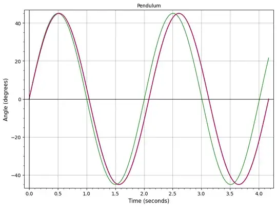
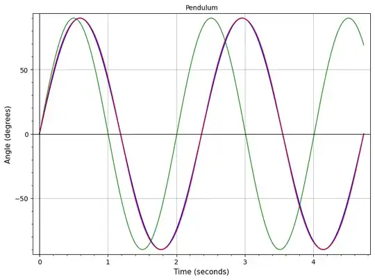
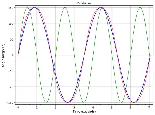
The program plots the true pendulum function in red. It can also plot the simple sine function (in green) or a sine function with its period corrected to the true period (in blue).
For smallish $\theta_m$, it's hard to see the difference between the true curve and the simple sines. Even for angles approaching $90°$, the period-corrected sine is still quite close to the true curve. Here are a few examples for a pendulum of length $1$ m.