In the calculus of variations, particularly Lagrangian mechanics, people often say we vary the position and the velocity independently. But velocity is the derivative of position, so how can you treat them as independent variables?
Asked
Active
Viewed 1.9k times
9 Answers
104
Unlike your question suggests, it is not true that velocity is varied independently of position. A variation of position $q \mapsto q + \delta q$ induces a variation of velocity $\partial_t q \mapsto \partial_t q + \partial_t (\delta q)$ as you would expect.
The only thing that may seem strange is that $q$ and $\partial_t q$ are treated as independent variables of the Lagrangian $L(q,\partial_t q)$. But this is not surprising; after all, if you ask "what is the kinetic energy of a particle?", then it is not enough to know the position of the particle, you also have to know its velocity to answer that question.
Put differently, you can choose position and velocity independently as initial conditions, that's why the Lagrangian function treats them as independent; but the calculus of variation does not vary them independently, a variation in position induces a fitting variation in velocity.
Greg Graviton
- 5,397
52
The answer to your main question is already given -- you do not vary coordiante and speed independently. But it seems that your main problem is about using coordinate and speed as independent variables.
Let me refer to this great book: "Applied Differential Geometry". By William L. Burke. The very first line of the book (where an author usually says to whom this book is devoted) is this:
It is true that from time to time student do ask this question. But attempts to explain it "top down" are usually just lead to more and more questions. One really needs to make mathematical "bottom up" order in the topic. Well, as the name of the book suggest -- the mathematical discipline one needs is differential geometry.
I cannot retell all the details, but briefly it looks like this:
- You start with a configuration space $M$ of your system. $M$ is a (differentiable) manifold, and $q$ are the coordinates on this manifold.
- Then there is a specific procedure, that allows you to add all the possible "speeds" at every given point of $M$. And you arrive at the tangent bundle $TM$, which is a manifold too, and ($q$,$\dot{q}$) are different coordinates on it.
- Lagrangian is a function on $TM$.
Kostya
- 20,288
33
Considering what Greg Graviton wrote, I'll write out the derivation and see if I can make sense of it.
$$ S = \int_{t_1}^{t_2} L(q, \dot q, t)\, \mathrm{d}t $$
where S is the action and L the Lagrangian. We vary the path and find the extremum of the action:
$$ \delta S = \int_{t_1}^{t_2} \left({\partial L \over \partial q}\delta q + {\partial L \over \partial \dot q}\delta \dot q\right) \,\mathrm{d}t = 0\,. $$
Here, q and $\dot q$ are varied independently. But then in the next step we use this identity,
$$ \delta \dot q = {\mathrm{d} \over \mathrm{d}t} \delta q. $$
And here is where the relationship between q and $\dot q$ enters the picture. I think that what is happening here is that q and $\dot q$ are treated as independent initially, but then the independence is removed by the identity.
$$ \delta S = \int_{t_1}^{t_2} \left({\partial L \over \partial q}\delta q + {\partial L \over \partial \dot q}{d \over \mathrm{d}t} \delta q\right) \,\mathrm{d}t = 0 $$
And then follows the rest of the derivation. We integrate the second term by parts:
$$ \delta S = \left[ {\partial L \over \partial \dot q}\delta q\right]_{t_1}^{t_2} + \int_{t_1}^{t_2} \left({\partial L \over \partial q} - {d \over dt}{\partial L \over \partial \dot q}\right)\delta q\, \mathrm{d}t = 0\,, $$
and the bracketed expression is zero because the endpoints are held fixed. And then we can pull out the Euler-Lagrange equation:
$$ {\partial L \over \partial q} - {\mathrm{d} \over \mathrm{d}t}{\partial L \over \partial \dot q} = 0\,. $$
Now it makes more sense to me. You start by treating the variables as independent but then remove the independence by imposing a condition during the derivation.
I think that makes sense. I expect in general other problems can be treated the same way.
(I copied the above equations from Mechanics by Landau and Lifshitz.)
grizzly adam
- 2,285
27
Here is my answer, which is basically an expanded version of Greg Graviton's answer.
The question of why one can treat position and velocity as independent variables arises in the definition of the Lagrangian $L$ itself, before one uses equation of motion, and before one thinks about varying the action $S:=\int_{t_i}^{t_f}\mathrm{d}t \ L$, and has therefore nothing to do with calculus of variation.
I) On one hand, let us first consider the role of the Lagrangian. Let there be given an arbitrary but fixed instant of time $t_0\in [t_i,t_f]$. The (instantaneous) Lagrangian $L(q(t_0),v(t_0),t_0)$ is a function of both the instantaneous position $q(t_0)$ and the instantaneous velocity $v(t_0)$ at the instant $t_0$. Here $q(t_0)$ and $v(t_0)$ are independent variables. Note that the (instantaneous) Lagrangian $L(q(t_0),v(t_0),t_0)$ does not depend on the past $t<t_0$ nor the future $t>t_0$. (One may object that the velocity profile $\dot{q}\equiv\dfrac{\mathrm{d}q}{\mathrm{d}t}:[t_i,t_f]\to\mathbb{R}$ is the derivative of the position profile $q:[t_i,t_f]\to\mathbb{R}$, so how can $q(t_0)$ and $v(t_0)$ be truly independent variables? The point is that since the equation of motion is of 2nd order, one is still entitled to make 2 independent choices of initial conditions: 1 initial position and 1 initial velocity.) We can repeat this argument for any other instant $t_0\in[t_i,t_f]\,.$
II) On the other hand, let us consider calculus of variation. The action functional $$S[q] ~:=~ \int_{t_i}^{t_f}\mathrm{d}t \ L(q(t),\dot{q}(t),t)\tag{1}$$ depends on the whole (perhaps virtual) path $q:[t_i,t_f]\to\mathbb{R}$. Here the time derivative $\dot{q}\equiv\dfrac{\mathrm{d}q}{\mathrm{d}t}$ does depend on the function $q:[t_i,t_f]\to \mathbb{R}\,.$ Extremizing the action functional
$$\begin{align}0~=~&\delta S \cr ~=~& \int_{t_i}^{t_f}\mathrm{d}t\left[\left.\frac{\partial L(q(t),v(t),t)}{\partial q(t)}\right|_{v(t)=\dot{q}(t)} \delta q(t) \right.\cr &+\left.\left.\frac{\partial L(q(t),v(t),t)}{\partial v(t)}\right|_{v(t)=\dot{q}(t)}\delta \dot{q}(t)\right]\cr ~=~& \int_{t_i}^{t_f}\mathrm{d}t\left[\left.\frac{\partial L(q(t),v(t),t)}{\partial q(t)}\right|_{v(t)=\dot{q}(t)} \delta q(t) \right.\cr &+\left.\left.\frac{\partial L(q(t),v(t),t)}{\partial v(t)}\right|_{v(t)=\dot{q}(t)}\frac{\mathrm d}{\mathrm{d}t}\delta q(t)\right]\cr ~=~& \int_{t_i}^{t_f}\mathrm{d}t\left[\left.\frac{\partial L(q(t),v(t),t)}{\partial q(t)}\right|_{v(t)=\dot{q}(t)} \right.\cr &-\left. \frac{\mathrm d}{\mathrm{d}t}\left(\left.\frac{\partial L(q(t),v(t),t)}{\partial v(t)}\right|_{v(t)=\dot{q}(t)} \right)\right]\delta q(t)\cr &+ \int_{t_i}^{t_f}\mathrm{d}t\frac{\mathrm{d}}{\mathrm{d}t}\left[\left.\frac{\partial L(q(t),v(t),t)}{\partial v(t)}\right|_{v(t)=\dot{q}(t)}\delta q(t)\right] \end{align}\tag{2} $$
with appropriate boundary conditions leads to Euler-Lagrange (EL) equation, which is the equation of motion (EOM).
$$ \begin{align} \frac{\mathrm d}{\mathrm{d}t}&\left(\left.\frac{\partial L(q(t),v(t),t)}{\partial v(t)} \right|_{v(t)=\dot{q}(t)} \right)\cr &~=~ \left.\frac{\partial L(q(t),v(t),t)}{\partial q(t)} \right|_{v(t)=\dot{q}(t)} ~.\tag{3}\label{eq:3}\end{align} $$
III) Note that
$$\frac{\mathrm{d}}{\mathrm{d}t}~=~\dot{v}(t)\frac{\partial}{\partial v(t)}+\dot{q}(t)\frac{\partial}{\partial q(t)}+\frac{\partial}{\partial t} \tag{4}$$
is a total time derivative, not an explicit time derivative $\dfrac{\partial}{\partial t}$, so that the EL equation $\eqref{eq:3}$ is really a 2nd-order ordinary differential equation (ODE),
$$\begin{align} \left(\ddot{q}(t)\frac{\partial}{\partial v(t)} +\dot{q}(t)\frac{\partial}{\partial q(t)} \right.&\left. +\frac{\partial}{\partial t}\right) \left. \frac{\partial L(q(t),v(t),t)}{\partial v(t)} \right|_{v(t)=\dot{q}(t)} \cr ~=~& \left.\frac{\partial L(q(t),v(t),t)}{\partial q(t)} \right|_{v(t)=\dot{q}(t)}~. \tag{5}\end{align}$$
To solve for the path $q:[t_i,t_f]\to \mathbb{R}$, one should specify two initial conditions, e.g., $$q(t_i)~=~q_i\qquad\text{and} \qquad\dot{q}(t_i)~=~v_i.\tag{6}$$
11
While it is true that the function $\dot{q}(t)$ is the derivative of the function $q(t)$ w.r.t. time, it is not true that the value $\dot{q}$ is at all related to the value $q$ at a given point in time, since a value is just a number, not a function. The action is a functional of $q(t)$, and so it would make no sense to vary the action both w.r.t. $q$ and $\dot{q}$. But the Lagrangian $L(q,\dot{q})$ is a function of the values $q$ and $\dot{q}$, not a functional of the functions $q(t)$ and $\dot{q}(t)$. We can promote $L$ to a function of time if we plug in $q(t)$ and $\dot{q}(t)$ instead of just $q$ and $\dot{q}$. (Remember a functional turns a function into a number, e.g., $S[q]$, whereas a function turns a value into a number, e.g., $L(q,\dot{q})$.
To solve for $q(t)$ we extremize the action $S$, by demanding that it is extremal at every point, $t$. This is equivalent to solving the Euler-Lagrange equations at every point $t$. Since at any point $t$ the values $q$ and $\dot{q}$ are independent, they can be varied independently.
davyjones
- 125
- 4
5
If we have a function $f(x,v)$, the partial derivatives are defined by $$\frac{\partial f(x,v)}{\partial x} \equiv \lim_{h\to 0} \frac{f(x+h,v)-f(x,v)}{h}$$ and $$\frac{\partial f(x,v)}{\partial v} \equiv \lim_{h\to 0} \frac{f(x,v+h)-f(x,v)}{h}$$ This implies, for example, for $f=v^2$ that $$\frac{\partial v^2}{\partial x} \equiv \lim_{h\to 0} \frac{v^2-v^2}{h} =0.$$ Moreover, for $v= \frac{dx}{dt}$ we find that $x \to x+h$ implies $v = \frac{dx}{dt} \to v' = \frac{d(x+h)}{dt} = \frac{dx}{dt} =v$. Thus $$\frac{\partial \frac{dx}{dt}^2}{\partial x} \equiv \lim_{h\to 0} \frac{\frac{dx}{dt}^2-\frac{dx}{dt}^2}{h} =0.$$ Hence it makes sense to consider the partial derivatives of the Lagrangian with respect to $x$ and $v$ separately and in this sense treat them independently.
In more physical terms, recall that our goal in the Lagrangian formalism is to figure out the correct path in configuration space between two fixed location. A path is characterized by a location and velocity at each point in time. We are as general as possible and consider really all possible paths. This implies that we consider all possible pairings of locations and velocities. The physical classical path is special for two reasons:
- it's a solution of the Euler-Lagrange equation (= extremum of the action)
- the locations and velocities at each moment in time are related by $v \equiv \frac{dq}{dt}$. (If you want, $v \equiv \frac{dq}{dt}$ is the second equation that we need in the Lagrangian formalism analogous to how there are two Hamilton equations in the Hamiltonian formalism. The second Hamilton equation defines the canonical momentum as a derivative of the Lagrangian. For general paths in phase space, any pairing of location and momentum is possible. Only for the physical classical path we find canonical momentum values that are given as the appropriate derivative of the Lagrangian.)
jak
- 10,431
4
The derivative of a function $f(t)$ is the function $\dot{f}(t)$ in general different than $f$, and in the general case the two are not even linearly dependent, which is simple to see if you take the Taylor expansion. It is only after you define differential equations with them that they are linked algebraically, and this is what the calculus of variations does.
auxsvr
- 2,407
1
I want to start with asserting that nowhere in the evaluation there is a stage where the two factors $y$ and $\tfrac{dy}{dx}$ are treated as independent.
The purpose of this answer is to address the question:
What does it mean that the differentiation of the Lagrangian is declared as partial differentiation?
I will first work that out for a specific case, and and then I discuss how it generalizes to all cases.
As quintessential example of application of calculus of variations I use the catenary problem.
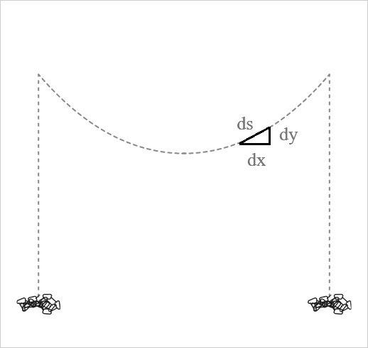
In the image the dashed line represents a chain that is free to move over two suspension points. I will refer to the curved part as 'the catenary' and I will refer to the vertical hanging part as 'the counterweight'. Let there be a small amount of friction, just enough friction to dissipate energy.
If the chain is released from a height slightly above the height represented in the diagram, then it will sag until it reaches a point of minimum potential energy.
Recapitulating the variational approach:
The goal is to obtain a function that gives the y-coordinate (vertical) as a function of the x-coordinate (horizontal)
For simplicity of the expressions I set the mass per unit of length to a value of 1, and I set the gravitational acceleration to a value of 1.
We set up the expression for the potential energy of the line element from coordinate $x$ to coordinate $(x + dx)$
$$ (ds)^2 = (dx)^2 + (dy)^2 \tag{1} $$
$$ ds = \sqrt{(dx)^2 + (dy)^2} \tag{2} $$
$$ ds = \sqrt{1 + \left(\tfrac{dy}{dx}\right)^2} \ dx \tag{3} $$
Hence the integral of the potential energy from suspension point $p_1$ to suspension point $p_2$ is:
$$ \int_{p_1}^{p_2} y \ \sqrt{1 + y'^2 } \ dx \tag{4} $$
That is, for every section $dx$ along the horizontal the potential energy of the line element is given by the product of the height $y$ and the length $ds$ (with the length $ds$ a function of the slope of the curve).
At this point I want to emphasize something about sweeping out variation: there is no degree of freedom available to vary $y$ and $\tfrac{dy}{dx}$ independently.
The variation is exclusively variation in the vertical direction; There is no freedom to introduce a variation component in the horizontal direction.
So: even though the catenary problem has two spatial degrees of freedom, horizontal and vertical, the variation is variation of the vertical coordinate only.
-When you raise the chain the height and the slope change together.
-When you allow the chain to sag the height and the slope change together.
The crucial thing is:
When the chain is not at the equilibrium point then as you raise/lower the chain either of the height/slope contributions is changing faster than the other.
The equilibrium point is a cross-over point. At the point where the chain is at equilibrium point the two contributions change at the same rate.
To compare the rate-of-change of the respective contributions we must take the derivative with respect to the vertical coordinate, since the variation is variation of the vertical coordinate. That is: the differential operator to be used is $\tfrac{d}{dy}$
(5) expresses that comparison, for the integrand $y \cdot \sqrt{1 + y'^2 }$ of (4)
$$ \left(\frac{d}{dy}y \right) \cdot \sqrt{1 + y'^2 } = y \cdot \left(\frac{d}{dy} \sqrt{1 + y'^2 } \right) \tag{5} $$
((5) is in very compact notation. Another option is to write (5) according to $y = f(x)$
$$ \left(\frac{d}{dy}f(x) \right) \cdot \sqrt{1 + \left(\frac{f(x)}{dx}\right)^2 } = f(x) \cdot \left(\frac{d}{dy} \sqrt{1 + \left(\frac{f(x)}{dx}\right)^2 } \right) \tag{6} $$
To keep the notation compact I will stay with the notation of (5).)
In (5) we have that on the left hand side the height factor is differentiated with respect to the vertical coordinate, and on the right hand side the slope factor is differentiated with respect to the vertical coordinate.
The next step (for the purpose of demonstrating the connection with the Euler-Lagrange equation) is to rearrange the differentiation on the right hand side of (5).
The following two differential operations are mathematically equivalent:
$$ \frac{df(y')}{dy} \Leftrightarrow \frac{d\left( \frac{d f(y')}{d(y')} \right)}{dx} \tag{7} $$
One way to corroborate that the two are equivalent is to insert $\tfrac{1}{2}\left(\tfrac{dy}{dx} \right)^2$ into both sides:
Left hand side:
$$ \frac{d\left(\tfrac{1}{2}(y')^2\right)}{dy} = \tfrac{1}{2}\left(2 y' \frac{d(y')}{dy}\right) = \frac{dy}{dx}\frac{d(y')}{dy} = \frac{d(y')}{dx} = \frac{d^2y}{dx^2} \tag{8} $$
Right hand side:
$$ \frac{d}{dx}\left( \frac{d \left(\tfrac{1}{2}(y')^2\right)}{d(y')} \right) = \frac{d}{dx}(y') = \frac{d^2y}{dx^2} \tag{9} $$
(8) and (9) both evaluate to $\tfrac{d^2y}{dx^2}$. While not a rigorous proof I submit this is sufficient corroboration.
(For another corroboration: scroll to the end of this answer)
Rearranging the differentiation according to (7) makes it possible to express relation (5) in partial differentiation notation:
$$ \frac{\partial (y \cdot \sqrt{1 + y'^2 })}{\partial y} = \frac{d}{dx}\frac{\partial (y \cdot \sqrt{1 + y'^2 })}{\partial (y')} \tag{9} $$
This property generalizes to any Lagrangian $L$
$$ \frac{\partial L}{\partial y} = \frac{d}{dx}\frac{\partial L}{\partial (y')} \tag{10} $$
Which is the Euler-Lagrange equation:
$$ \frac{\partial L}{\partial y} - \frac{d}{dx}\frac{\partial L}{\partial (y')} = 0 \tag{11} $$
Discussion
The objective of this answer is to address the question:
"What does it mean that the differentiation of the Lagrangian is declared as partial differentiation?"
I submit that the partial differentiation notation is a hack. The key equation is (5): the comparison equation, which does not lend itself to partial differentiation notation.
It just so happens that the differentiation can be rearranged to slot in with partial differentiation notation.
The catenary problem has the following property: if you take a subsection of the curve: that subsection is an instance of the catenary problem too.
You can keep subdividing indefinitely; every subsection of the curve, down to infinitisimally short subsections, is an instance of the catenary problem.
The equilibrium property that is expressed in (5) obtains at the infinitesimal level, and from there it propagates out to the curve as whole.
This infinitesimal property is the defining characteristic that allows a problem to be solved with calculus of variations.
Further reading:
Preetum Nakkiran:
Geometric derivation of the Euler-Lagrange equation
Preetum Nakkiran capitalizes on the fact that the Euler-Lagrange equation is a differential equation.
The Euler-Lagrange equation can be derived with purely differential reasoning.
(More extensive discussion of calculus of variations is available on my own website. A link to my website is available on my stackexchange profile page.)
Appendix:
Another way to corroborate (7).
The left hand side of (7):
$$ \frac{df(y')}{dy} \tag{A.1} $$
Apply the chain rule, and write the result in Leibniz notation for the chain rule: a product of two differentations:
$$ \frac{dy'}{dy} \cdot \frac{df(y')}{dy'} \tag{A.2} $$
If it is granted that (A.3) is reasonable then (A.1) can be restated accordingly:
$$ \frac{d\left(\tfrac{dy}{dx}\right)}{dy} \stackrel{?}{=} \frac{d}{dx} \tag{A.3} $$
$$ \frac{df(y')}{dy} \Leftrightarrow \frac{d}{dx}\left(\frac{df(y')}{dy'} \right) \tag{A.4} $$
Cleonis
- 24,617
1
After reading all the answers rigorously, I came up with a simple explanation. The Lagranian $L(q,\dot{q},t)$ has no notion of path, only of the values $q,\dot{q}$. At each instant "$t$", the values $q$ and $\dot{q}$ can be varied independently to produce some contribution to S. But only a set of values {$q,\dot{q}$} will extremize this action S. This set is given by {$q(t),\dot{q}(t)$}, the solutions to the Euler Lagrange equations. Of course, on this path they are dependent.
The notation can cause some confusion and it might help to just write L($\alpha, \beta$,t) where $\alpha, \beta$ are values that can be varied independently. Requiring that ${\frac{d}{dt}\alpha} = {\beta}$ and that the action S be minimized will yield the Euler Lagrange equations which will give a set of values {$\alpha(t), \beta(t)$} which we can define as {$q(t),\dot{q(t)}$}
qubitz
- 425