$\texttt{ELECTRIC FIELD LINES BETWEEN TWO OPPOSITELY CHARGED POINT CHARGES}$
$=\!=\!=\!=\!=\!=\!=\!=\!=\!=\!=\!=\!=\!=\!=\!=\!=\!=\!=\!=\!=\!=\!=\!=\!=\!=\!=\!=\!=\!=\!=\!=\!=\!=\!=\!=\!=\!=\!=\!=\!=\!=\!=\!=\!=\!=\!=\!=\!=\!=\!=\!=\!=\!=\!=\!=\!=\!=\!=\!=\!=\!=\!=\!$
$\boldsymbol\S$ 1. Summary of general results
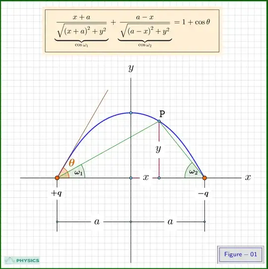
Using the $''$unusual technique$''$ of Michael Seifert's answer, essentially an interesting application of Gauss Law, we provide an implicit equation for the electric field line between two oppositely charged point charges $\,+q,-q\,$ that forms an angle $\,\theta\,$ with respect to the line joint the two charges at its starting point $\,+q\,$ as shown in Figure-01.
The implicit equation of this electric field line is
\begin{equation}
\dfrac{x\boldsymbol+a}{\sqrt{\left(x\boldsymbol+a\right)^2\boldsymbol+y^2}}\boldsymbol+\dfrac{a\boldsymbol-x}{\sqrt{\left(a\boldsymbol-x\right)^2\boldsymbol+y^2}}\boldsymbol=1\boldsymbol+\cos\theta
\tag{01}\label{01}
\end{equation}
expressed also as
\begin{equation}
\cos\omega_1\boldsymbol+\cos\omega_2\boldsymbol=1\boldsymbol+\cos\theta
\tag{02}\label{02}
\end{equation}
where $\,\omega_1,\omega_2\,$ the angles shown in Figure-01.
Equation \eqref{02} is used to sketch this curve with precision. More exactly we use the angle $\,\omega_1\,$ as a variable parameter in the range $\,\left[0,\theta\right]$. First we draw a line from point $\,+q\,$ at angle $\,\omega_1\,$ with respect to the $\,x\boldsymbol-$axis. Second we draw a line from point $\,-q\,$ at angle $\,\omega_2\boldsymbol=\arccos\left(1\boldsymbol+\cos\theta\boldsymbol-\cos\omega_1\right)\,$ with respect to the $\,x\boldsymbol-$axis. These two lines intersect at point $\,\texttt P$. Varying $\,\omega_1\,$ in the range $\,\left[0,\theta\right]\,$ (by a tool called animation) and moving point $\,\texttt P$ leaving its trace behind it (by a tool called trace on) the curve is drawn with precision. Using this approach we find a parametric representation of the curve provided in $\boldsymbol\S$ 5.
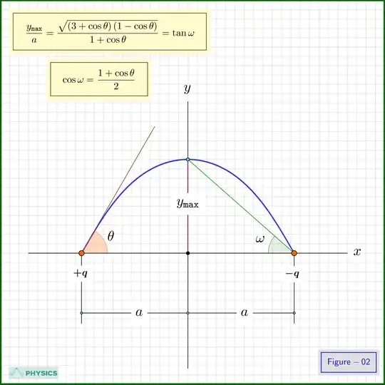
Because of symmetry we meet the maximum height $\,y_{\texttt{max}}\,$ at $\,x\boldsymbol=0$, so from equation \eqref{01}
\begin{equation}
\dfrac{2a}{\sqrt{a^2\boldsymbol+y^2_{\texttt{max}}}}\boldsymbol=1\boldsymbol+\cos\theta \qquad\boldsymbol\implies
\nonumber
\end{equation}
\begin{equation}
\dfrac{y_{\texttt{max}}}{a}\boldsymbol=\dfrac{\sqrt{\left(3\boldsymbol+\cos\theta\right)\left(1\boldsymbol-\cos\theta\right)}}{1\boldsymbol+\cos\theta}\boldsymbol=\tan\omega
\tag{03}\label{03}
\end{equation}
while equation \eqref{02} with $\,\omega_1\boldsymbol=\omega\boldsymbol=\omega_2\,$ yields
\begin{equation}
\cos\omega\boldsymbol=\dfrac{1\boldsymbol+\cos\theta}{2}
\tag{04}\label{04}
\end{equation}
see Figure-02.
$=\!=\!=\!=\!=\!=\!=\!=\!=\!=\!=\!=\!=\!=\!=\!=\!=\!=\!=\!=\!=\!=\!=\!=\!=\!=\!=\!=\!=\!=\!=\!=\!=\!=\!=\!=\!=\!=\!=\!=\!=\!=\!=\!=\!=\!=\!=\!=\!=\!=\!=\!=\!=\!=\!=\!=\!=\!=\!=\!=\!=\!=\!=\!$
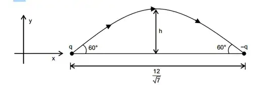
$\boldsymbol\S$ 2. The special case $\,\theta\boldsymbol=60^\circ, 2a\boldsymbol=12/\sqrt{7}$
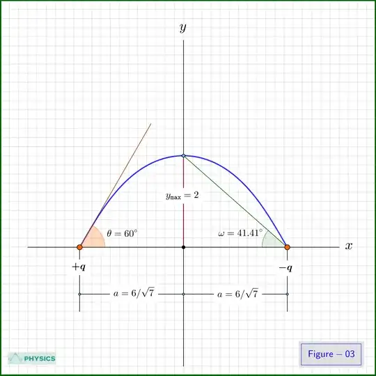
Inserting above data in equation \eqref{03} we find
\begin{equation}
y_{\texttt{max}}\boldsymbol=2\,,\qquad \omega\boldsymbol=41.41^\circ
\tag{05}\label{05}
\end{equation}
see Figure-03.
$=\!=\!=\!=\!=\!=\!=\!=\!=\!=\!=\!=\!=\!=\!=\!=\!=\!=\!=\!=\!=\!=\!=\!=\!=\!=\!=\!=\!=\!=\!=\!=\!=\!=\!=\!=\!=\!=\!=\!=\!=\!=\!=\!=\!=\!=\!=\!=\!=\!=\!=\!=\!=\!=\!=\!=\!=\!=\!=\!=\!=\!=\!=\!$
$\boldsymbol\S$ 3. The Proof of equations \eqref{01}, \eqref{02}
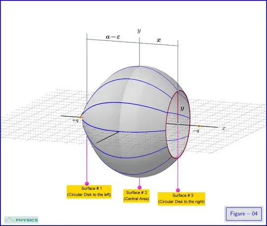
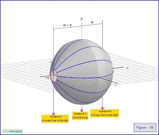
To prove equation \eqref{01} or equivalently \eqref{02} we apply Gauss Law to the closed surface shown from two different angles in Figures-04 and -05 in the limit $\,\varepsilon \boldsymbol\rightarrow 0$. More precisely this closed surface is produced as follows : the closed surface generated in space from a complete revolution of the electric flux line in Figure-01 around the $\,x\boldsymbol-$axis is intersected by two planes normal to this axis. A first plane on a general coordinate $\,x\,$ which produces the circular intersection of radius $\,y\,$ shown in Figure-04 (Surface $\#$3 - Circular Disk to the right) and a second plane at a very small distance $\,\varepsilon \,$ to the right of the the charge $\,+q\,$ which produces the circular intersection of very small radius shown in Figure-05 (Surface $\#$1 - Circular Disk to the left).
3D-Drawing of surfaces in GeoGebra using tools "Trace On" and "Animation ON" : Trajectory of electric field lines Fig A04 Animation GeoGebra.
The closed surface of above Figures doesn't include electric charge. So, by Gauss Law the net electric flux through it will be zero. That is
\begin{equation}
\Phi_1\left(\varepsilon\right)\boldsymbol+\Phi_2\boldsymbol+\Phi_3\boldsymbol=0
\tag{06}\label{06}
\end{equation}
where $\,\Phi_1\left(\varepsilon\right)\,$ the flux through the Surface $\#$1 (the Circular Disk to the left) a function of the small distance $\,\varepsilon$, $\,\Phi_2\,$ the flux through the Surface $\#$2 (the Central Area) and $\,\Phi_3\,$ the flux through the Surface $\#$3 (the Circular Disk to the right).
At any point of the Surface $\#$2 the electric field intensity $\,\mathbf E\,$ is tangent to the surface so
\begin{equation}
\Phi_2\boldsymbol=0
\tag{07}\label{07}
\end{equation}
With respect to the Surface $\#$1 we split the flux $\,\Phi_1\left(\varepsilon\right)\,$ as follows
\begin{equation}
\Phi_1\left(\varepsilon\right)\boldsymbol=\Phi^{\boldsymbol+}_1\left(\varepsilon\right)\boldsymbol+\Phi^{\boldsymbol-}_1\left(\varepsilon\right)
\tag{08}\label{08}
\end{equation}
where $\,\Phi^{\boldsymbol+}_1\left(\varepsilon\right),\Phi^{\boldsymbol-}_1\left(\varepsilon\right)\,$ the flux produced by the point charges $\,+q,-q\,$ respectively. In the limit $\,\varepsilon \boldsymbol\rightarrow 0\,$ the solid angle of the Surface $\#$1 as seen from the charge $\,-q\,$ is zero, while as seen from the charge $\,+q\,$ is that on the apex of a cone of plane angle $\,\theta\,$ that is
\begin{equation}
\Theta\left(\theta\right)\boldsymbol=2\pi\left(1\boldsymbol-\cos\theta\right)
\tag{09}\label{09}
\end{equation}
so
\begin{equation}
\begin{split}
\Phi^{\boldsymbol+}_1 & \boldsymbol=\lim_{\varepsilon \boldsymbol\rightarrow 0}\Phi^{\boldsymbol+}_1\left(\varepsilon\right)\boldsymbol=\boldsymbol- \dfrac{\Theta\left(\theta\right)}{4\pi}\dfrac{q}{\epsilon_0}\boldsymbol=\boldsymbol-\dfrac{q}{2\epsilon_0}\left(1\boldsymbol-\cos\theta\right)\\
\Phi^{\boldsymbol-}_1 & \boldsymbol=\lim_{\varepsilon \boldsymbol\rightarrow 0}\Phi^{\boldsymbol-}_1\left(\varepsilon\right)\boldsymbol=0\\
\end{split}
\tag{10}\label{10}
\end{equation}
that is
\begin{equation}
\Phi_1\boldsymbol=\boldsymbol-\dfrac{q}{2\epsilon_0}\left(1\boldsymbol-\cos\theta\right)
\tag{11}\label{11}
\end{equation}
The minus sign is due to the fact that for $\,q\boldsymbol>0\,$ the flux is inwards to the closed surface.
Similarly, with respect to the Surface $\#$3 we split the flux $\,\Phi_3\,$ as follows
\begin{equation}
\Phi_3\boldsymbol=\Phi^{\boldsymbol+}_3\boldsymbol+\Phi^{\boldsymbol-}_3
\tag{12}\label{12}
\end{equation}
where $\,\Phi^{\boldsymbol+}_3,\Phi^{\boldsymbol-}_3\,$ the flux produced by the point charge $\,+q,-q\,$ respectively. The solid angle $\Theta\left(\omega_1\right)$ of the Surface $\#$3 as seen from the charge $\,+q\,$ is that on the apex of a cone of plane angle $\,\omega_1$, while the solid angle $\Theta\left(\omega_2\right)$ of the Surface $\#$3 as seen from the charge $\,-q\,$ is that on the apex of a cone of plane angle $\,\omega_2\,$, see Figure-01. So
\begin{equation}
\begin{split}
\Theta\left(\omega_1\right) & \boldsymbol=2\pi\left(1\boldsymbol-\cos\omega_1\right)\\
\Theta\left(\omega_2\right) & \boldsymbol=2\pi\left(1\boldsymbol-\cos\omega_2\right)\\
\end{split}
\tag{13}\label{13}
\end{equation}
and
\begin{equation}
\begin{split}
\Phi^{\boldsymbol+}_3 & \boldsymbol= \dfrac{\Theta\left(\omega_1\right)}{4\pi}\dfrac{q}{\epsilon_0}\boldsymbol=\dfrac{q}{2\epsilon_0}\left(1\boldsymbol-\cos\omega_1\right)\\
\Phi^{\boldsymbol-}_3 & \boldsymbol= \dfrac{\Theta\left(\omega_2\right)}{4\pi}\dfrac{q}{\epsilon_0}\boldsymbol=\dfrac{q}{2\epsilon_0}\left(1\boldsymbol-\cos\omega_2\right)\\
\end{split}
\tag{14}\label{14}
\end{equation}
So
\begin{equation}
\Phi_3\boldsymbol=\Phi^{\boldsymbol+}_3\boldsymbol+\Phi^{\boldsymbol-}_3\boldsymbol=\dfrac{q}{2\epsilon_0}\left(2\boldsymbol-\cos\omega_1\boldsymbol-\cos\omega_2\right)
\tag{15}\label{15}
\end{equation}
Now,
\begin{equation}
\Phi_1\boldsymbol+\Phi_3\boldsymbol=0 \quad \stackrel{\eqref{11},\eqref{15}}{\boldsymbol{=\!=\!=\!\Longrightarrow}} \quad \boldsymbol-\dfrac{q}{2\epsilon_0}\left(1\boldsymbol-\cos\theta\right)\boldsymbol+\dfrac{q}{2\epsilon_0}\left(2\boldsymbol-\cos\omega_1\boldsymbol-\cos\omega_2\right)\boldsymbol=0
\tag{16}\label{16}
\end{equation}
so proving equation \eqref{02}
\begin{equation}
\cos\omega_1\boldsymbol+\cos\omega_2\boldsymbol=1\boldsymbol+\cos\theta
\tag{02}
\end{equation}
But from Figure-01
\begin{equation}
\cos\omega_1\boldsymbol=\dfrac{x\boldsymbol+a}{\sqrt{\left(x\boldsymbol+a\right)^2\boldsymbol+y^2}}\,, \qquad \cos\omega_2\boldsymbol=\dfrac{a\boldsymbol-x}{\sqrt{\left(a\boldsymbol-x\right)^2\boldsymbol+y^2}}
\tag{17}\label{17}
\end{equation}
so proving equation \eqref{01}
\begin{equation}
\dfrac{x\boldsymbol+a}{\sqrt{\left(x\boldsymbol+a\right)^2\boldsymbol+y^2}}\boldsymbol+\dfrac{a\boldsymbol-x}{\sqrt{\left(a\boldsymbol-x\right)^2\boldsymbol+y^2}}\boldsymbol=1\boldsymbol+\cos\theta
\tag{01}
\end{equation}
$=\!=\!=\!=\!=\!=\!=\!=\!=\!=\!=\!=\!=\!=\!=\!=\!=\!=\!=\!=\!=\!=\!=\!=\!=\!=\!=\!=\!=\!=\!=\!=\!=\!=\!=\!=\!=\!=\!=\!=\!=\!=\!=\!=\!=\!=\!=\!=\!=\!=\!=\!=\!=\!=\!=\!=\!=\!=\!=\!=\!=\!=\!=\!$
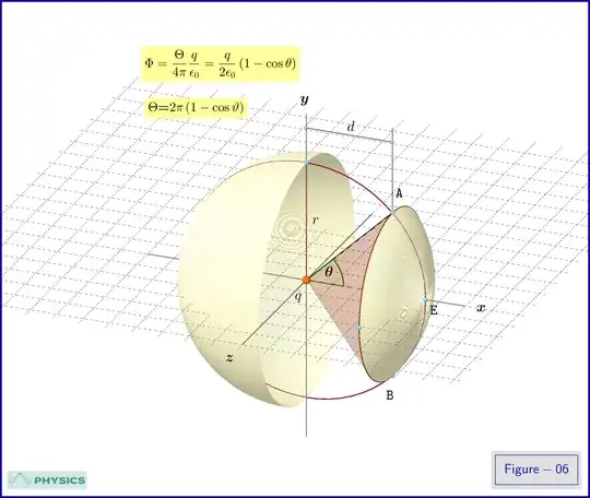
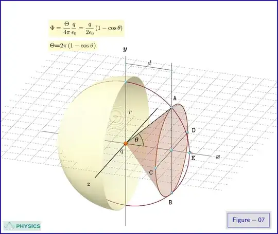
$\boldsymbol\S$ 4. Spherical Caps : Solid Angle and Electric Flux
For the surface area of the spherical cap $\,\texttt{AEB}\,$ shown in Figure-06 we have
\begin{equation}
S_\texttt{AEB}\boldsymbol=2\pi\,r^2\left(1\boldsymbol-\cos\theta\right)
\tag{18}\label{18}
\end{equation}
The proof provided by integration could be found in many textbooks, in the web and also in many answers in PSE herein.
So for the solid angle $\,\Theta\,$ by which this spherical cap is seen from the center of the sphere
\begin{equation}
\Theta\boldsymbol=\dfrac{S_\texttt{AEB}}{r^2}\boldsymbol=2\pi\left(1\boldsymbol-\cos\theta\right)
\tag{19}\label{19}
\end{equation}
and for the electric flux due to a point charge $\,q\,$ on the center
\begin{equation}
\Phi_\texttt{AEB}\boldsymbol=\dfrac{\Theta}{4\pi}\dfrac{q}{\epsilon_0}\boldsymbol=\dfrac{q}{2\epsilon_0}\left(1\boldsymbol-\cos\theta\right)
\tag{20}\label{20}
\end{equation}
For the circular disk $\,\texttt{ACBD}\,$ shown in Figure-07, in a sense the $''$base$''$ of the spherical cap $\,\texttt{AEB}\,$ shown in Figure-06, the solid angle and the electric flux are identical to those of the latter as given by equations \eqref{19} and \eqref{20} respectively.
$=\!=\!=\!=\!=\!=\!=\!=\!=\!=\!=\!=\!=\!=\!=\!=\!=\!=\!=\!=\!=\!=\!=\!=\!=\!=\!=\!=\!=\!=\!=\!=\!=\!=\!=\!=\!=\!=\!=\!=\!=\!=\!=\!=\!=\!=\!=\!=\!=\!=\!=\!=\!=\!=\!=\!=\!=\!=\!=\!=\!=\!=\!=\!$
$\boldsymbol\S$ 5. Revisiting the equation \eqref{01} of the Electric Field Line
As mentioned in $\boldsymbol\S$ 1 we could find a parametric representation of the electric field line shown in Figure-01, as follows : The point $\,\texttt P\,$ is the intersection of two lines, the first one through the point charge $\,+q\,$ at angle $\,\omega_1\,$ and a second one through the point charge $\,-q\,$ at angle $\,\omega_2\,$ with respect to the line joining the two charges. These lines are represented by the equations
\begin{align}
y \boldsymbol- x \tan\omega_1 & \boldsymbol= a\tan\omega_1
\tag{21a}\label{21a}\\
y \boldsymbol+ x \tan\omega_2 & \boldsymbol= a\tan\omega_2
\tag{21b}\label{21b}
\end{align}
respectively. Solving this system with respect to $\,x,y\,$ we find the coordinates of their intersection point $\,\texttt P$
\begin{equation}
\begin{split}
x & \boldsymbol=\dfrac{\tan\omega_2\boldsymbol-\tan\omega_1 }{\tan\omega_2\boldsymbol+\tan\omega_1}a\boldsymbol=\dfrac{\sin\left(\omega_2\boldsymbol-\omega_1\right) }{\sin\left(\omega_2\boldsymbol+\omega_1\right)}a\\
y & \boldsymbol=\dfrac{2\tan\omega_2\tan\omega_1 }{\tan\omega_2\boldsymbol+\tan\omega_1 }a\boldsymbol=\dfrac{2\sin\omega_2\sin\omega_1 }{\sin\left(\omega_2\boldsymbol+\omega_1\right)}a\\
\end{split}
\tag{22}\label{22}
\end{equation}
But from equation \eqref{02}
\begin{equation}
\omega_2\boldsymbol=\arccos\left(1\boldsymbol+\cos\theta\boldsymbol-\cos\omega_1\right)
\tag{23}\label{23}
\end{equation}so we have the following $\,\omega_1\boldsymbol-$parametric equation \begin{equation}
\begin{split}
x \boldsymbol=\dfrac{\tan\left[\arccos\left(1\boldsymbol+\cos\theta\boldsymbol-\cos\omega_1\right)\right]\boldsymbol-\tan\omega_1 }{\tan\left[\arccos\left(1\boldsymbol+\cos\theta\boldsymbol-\cos\omega_1\right)\right]\boldsymbol+ \tan\omega_1}a\\
y \boldsymbol=\dfrac{2\tan\left[\arccos\left(1\boldsymbol+\cos\theta\boldsymbol-\cos\omega_1\right)\right]\tan\omega_1 }{\tan\left[\arccos\left(1\boldsymbol+\cos\theta\boldsymbol-\cos\omega_1\right)\right]\boldsymbol+ \tan\omega_1}a\\
\end{split}
\tag{24}\label{24}
\end{equation}
that is
\begin{equation}
\begin{split}
\dfrac{x}{a} & \boldsymbol=\dfrac{\cos\omega_1\sqrt{\left(2\boldsymbol+\cos\theta\boldsymbol-\cos\omega_1\right)\left(\cos\omega_1\boldsymbol-\cos\theta\right)}\boldsymbol-\sin\omega_1\left(1\boldsymbol+\cos\theta\boldsymbol-\cos\omega_1\right) }{\cos\omega_1\sqrt{\left(2\boldsymbol+\cos\theta\boldsymbol-\cos\omega_1\right)\left(\cos\omega_1\boldsymbol-\cos\theta\right)}\boldsymbol+\sin\omega_1\left(1\boldsymbol+\cos\theta\boldsymbol-\cos\omega_1\right)}\\
\dfrac{y}{a} & \boldsymbol=\dfrac{2\sqrt{\left(2\boldsymbol+\cos\theta\boldsymbol-\cos\omega_1\right)\left(\cos\omega_1\boldsymbol-\cos\theta\right)}\sin\omega_1}{\cos\omega_1\sqrt{\left(2\boldsymbol+\cos\theta\boldsymbol-\cos\omega_1\right)\left(\cos\omega_1\boldsymbol-\cos\theta\right)}\boldsymbol+\sin\omega_1\left(1\boldsymbol+\cos\theta\boldsymbol-\cos\omega_1\right)}\\
& \hphantom{------------}\omega_1 \in \left[0,\theta\right]\\
\end{split}
\tag{25}\label{25}
\end{equation}
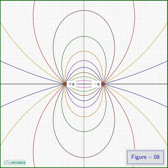
In Figure-08 the curves for $\,\theta\boldsymbol=k\pi/12, k=1,2,3\cdots 11\,$ are shown.