$\newcommand{\bl}[1]{\boldsymbol{#1}}
\newcommand{\e}{\bl=}
\newcommand{\p}{\bl+}
\newcommand{\m}{\bl-}
\newcommand{\mb}[1]{\mathbf {#1}}
\newcommand{\mc}[1]{\mathcal {#1}}
\newcommand{\mr}[1]{\mathrm {#1}}
\newcommand{\mf}[1]{\mathfrak{#1}}
\newcommand{\gr}{\bl>}
\newcommand{\les}{\bl<}
\newcommand{\greq}{\bl\ge}
\newcommand{\leseq}{\bl\le}
\newcommand{\il}[1]{$\:#1\:$}
\newcommand{\plr}[1]{\left(#1\right)}
\newcommand{\blr}[1]{\left[#1\right]}
\newcommand{\clr}[1]{\left\{#1\right\}}
\newcommand{\vlr}[1]{\left\vert#1\right\vert}
\newcommand{\Vlr}[1]{\left\Vert#1\right\Vert}
\newcommand{\lara}[1]{\left\langle#1\right\rangle}
\newcommand{\lav}[1]{\left\langle#1\right|}
\newcommand{\vra}[1]{\left|#1\right\rangle}
\newcommand{\lavra}[2]{\left\langle#1|#2\right\rangle}
\newcommand{\lavvra}[3]{\left\langle#1\right|#2\left|#3\right\rangle}
\newcommand{\vp}{\vphantom{\dfrac{a}{b}}}
\newcommand{\Vp}[1]{\vphantom{#1}}
\newcommand{\hp}[1]{\hphantom{#1}}
\newcommand{\tl}[1]{\tag{#1}\label{#1}}$
ANSWER$\bl{\m01}$
(2.b) The magnetic field lines formed between two parallel wires when the electrical currents are flowing in the opposite direction.
The differential equation to be solved is
\begin{equation}
\dfrac{\mr dy}{\mr dx} \e \dfrac{B_y\plr{x,y}}{B_x\plr{x,y}}
\tl{01}
\end{equation}
By a first glance it seems to be difficult or may be impossible to succeed separation of the used variables $\:\plr{x,y}$. We will solve this equation by a proper change of variables. The new variables are
\begin{equation}
u \e \tan\theta_{\mr A} \,,\qquad v \e \tan\theta_{\mr B}
\tl{02}
\end{equation}
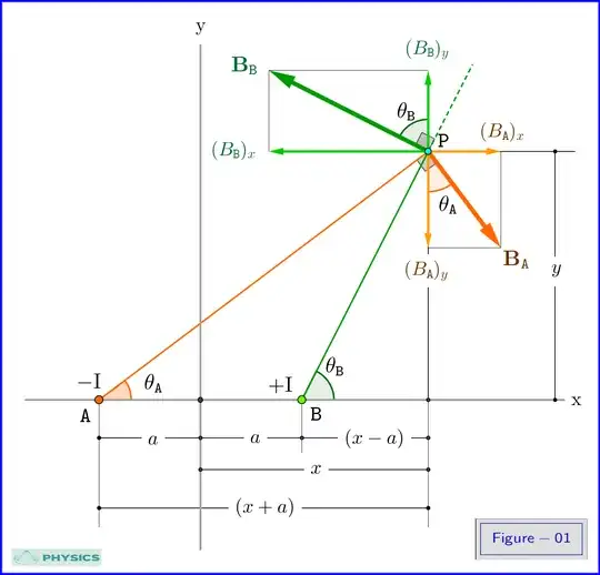
where $\:\plr{\theta_{\mr A},\theta_{\mr B}}\:$ the angles shown in Figure-01 .
Using the geometry of the problem we'll transform the differential equation \eqref{01} with respect to $\:\plr{x,y}\:$ to a differential equation with respect to $\:\plr{ u, v}$. The new differential equation is separable and we note a priori that its solution yields the result
\begin{equation}
\sin\theta_{\mr B} \e \lambda \sin\theta_{\mr A}
\nonumber
\end{equation}
where $\:\lambda\:$ a constant factor. To each permissible value of $\:\lambda\:$ there corresponds a magnetic field line.
At first from the geometry of the problem we have
\begin{equation}
\plr{x \m a}\tan\theta_{\mr B} \e y \e \plr{x \p a}\tan\theta_{\mr A}
\nonumber
\end{equation}
or
\begin{equation}
\plr{x \m a} v \e y \e \plr{x \p a} u
\tl{03}
\end{equation}
so
\begin{equation}
x \e \dfrac{\tan\theta_{\mr B}\p\tan\theta_{\mr A}}{\tan\theta_{\mr B}\m\tan\theta_{\mr A}}\, a \,,\qquad y \e \dfrac{2\tan\theta_{\mr B} \tan\theta_{\mr A}}{\tan\theta_{\mr B} \m \tan\theta_{\mr A}}\, a
\tl{04}
\end{equation}
or
\begin{equation}
x \e \plr{\dfrac{v\p u}{v\m u}} a \,,\qquad y \e \plr{\dfrac{2\,v\, u}{v \m u}} a
\tl{05}
\end{equation}
From \eqref{05}
\begin{equation}
\mr dx \e 2\,\dfrac{v\mr du\m u\mr d v}{\plr{v\m u}^2}\, a \,,\qquad \mr dy \e 2\,\dfrac{v^2\mr du\m u^2\mr d v}{\plr{v\m u}^2}\, a
\tl{06}
\end{equation}
From \eqref{06} the left hand side of \eqref{01} is transformed as follows
\begin{equation}
\dfrac{\mr dy}{\mr dx} \e \dfrac{v^2\mr du\m u^2\mr d v}{v\mr du\m u\mr d v}
\tl{07}
\end{equation}
For the transformation of the right hand side of \eqref{01} we have at first, see Figure-01,
\begin{align}
B_x & \e \plr{B_{\mr A}}_x\p \plr{B_{\mr B}}_x \e \dfrac{\mu_0 \mr I}{2\pi}\plr{\dfrac{\sin\theta_{\mr A}}{\mr{PA}} \m \dfrac{\sin\theta_{\mr B}}{\mr{PB}}}
\tl{08a}\\
B_y & \e \plr{B_{\mr A}}_y\p \plr{B_{\mr B}}_y\e \dfrac{\mu_0 \mr I}{2\pi}\plr{\dfrac{\cos\theta_{\mr B}}{\mr{PB}} \m \dfrac{\cos\theta_{\mr A}}{\mr{PA}}}
\tl{08b}
\end{align}
so
\begin{equation}
\dfrac{B_y}{B_x} \e \dfrac{\plr{\dfrac{\cos\theta_{\mr B}}{\mr{PB}} \m \dfrac{\cos\theta_{\mr A}}{\mr{PA}}}}{\plr{\dfrac{\sin\theta_{\mr A}}{\mr{PA}} \m \dfrac{\sin\theta_{\mr B}}{\mr{PB}}}}
\tl{09}
\end{equation}
From the geometry of the problem
\begin{equation}
\mr{PA} \e \dfrac{y}{\sin\theta_{\mr A}} \,,\qquad \mr{PB} \e \dfrac{y}{\sin\theta_{\mr B}}
\tl{10}
\end{equation}
and \eqref{09} yields
\begin{equation}
\begin{split}
\dfrac{B_y}{B_x} & \e \dfrac{\plr{\sin\theta_{\mr B}\cos\theta_{\mr B} \m \sin\theta_{\mr A}\cos\theta_{\mr A}}}{\plr{\sin^2\theta_{\mr A} \m \sin^2\theta_{\mr B}}}\\
&\e \dfrac{\plr{\dfrac{\tan\theta_{\mr B}}{\cos^2\theta_{\mr A}}\m{\dfrac{\tan\theta_{\mr A}}{\cos^2\theta_{\mr B}}}}}{\plr{\dfrac{\tan^2\theta_{\mr A}}{\cos^2\theta_{\mr B}}\m{\dfrac{\tan^2\theta_{\mr B}}{\cos^2\theta_{\mr A}}}}}\\
& \e \dfrac{\tan\theta_{\mr B}\plr{1\p\tan^2\theta_{\mr A}}\m\tan\theta_{\mr A}\plr{1\p\tan^2\theta_{\mr B}}}{\tan^2\theta_{\mr A}\plr{1\p\tan^2\theta_{\mr B}}\m\tan^2\theta_{\mr B}\plr{1\p\tan^2\theta_{\mr A}}} \\
& \e \dfrac{\tan\theta_{\mr A}\tan\theta_{\mr B}\m 1}{\tan\theta_{\mr A}\p\tan\theta_{\mr B}}\e\m\dfrac{1}{\tan\plr{\theta_{\mr A}\p\theta_{\mr B}}}\e \tan\blr{\plr{\theta_{\mr A}\p\theta_{\mr B}}\m\dfrac{\pi}{2}}\\
\end{split}
\tl{11}
\end{equation}
Replacing $\:\tan\theta_{\mr A},\tan\theta_{\mr B}\:$ with $\:u,v\:$ respectively
\begin{equation}
\dfrac{B_y}{B_x} \e \dfrac{u\,v \m 1}{u \p v}
\tl{12}
\end{equation}
Combining \eqref{01}, \eqref{07} and \eqref{12} we have the differential equation in terms of the new variables $\:u,v$
\begin{equation}
\dfrac{v^2\mr du\m u^2\mr d v}{v\mr du\m u\mr d v}\e \dfrac{u\,v \m 1}{u \p v}
\tl{13}
\end{equation}
or
\begin{equation}
\dfrac{\mr du}{u\plr{1\p u^2}} \e \dfrac{\mr dv}{v\plr{1\p v^2}}
\tl{14}
\end{equation}
that is
\begin{equation}
\dfrac{\mr d u^2}{ u^2}\m\dfrac{\mr d\plr{1\p u^2}}{\plr{1\p u^2}} \e \dfrac{\mr d v^2}{ v^2}\m\dfrac{\mr d\plr{1\p v^2}}{\plr{1\p v^2}}
\tl{15}
\end{equation}
which integrated yields
\begin{equation}
\ln\plr{\dfrac{u^2}{1\p u^2}} \e \ln\plr{\dfrac{v^2}{1\p v^2}}\p \texttt{constant}
\tl{16}
\end{equation}
But
\begin{equation}
\dfrac{u^2}{1\p u^2} \e \dfrac{\tan^2\theta_{\mr A}}{1\p \tan^2\theta_{\mr A}}\e \sin^2\theta_{\mr A}\,,\quad \dfrac{v^2}{1\p v^2} \e \dfrac{\tan^2\theta_{\mr B}}{1\p \tan^2\theta_{\mr B}}\e \sin^2\theta_{\mr B}
\tl{17}
\end{equation}
and equation \eqref{16} gives
\begin{equation}
\ln\plr{\sin^2\theta_{\mr A}} \e \ln\plr{\sin^2\theta_{\mr B}}\p \texttt{constant}^\prime
\tl{18}
\end{equation}
Because of symmetry with respect to the $\:\mr x\m$axis we consider that $\:\theta_{\mr A},\theta_{\mr B} \bl\in \plr{0,\pi}\:$ so $\:\sin\theta_{\mr A},\sin\theta_{\mr B} \gr 0\:$ and from \eqref{18}
\begin{equation}
\boxed{\:\:
\sin\theta_{\mr B} \e \lambda \sin\theta_{\mr A}\:\:\vp}
\tl{19}
\end{equation}
where $\:\lambda\:$ a constant factor.
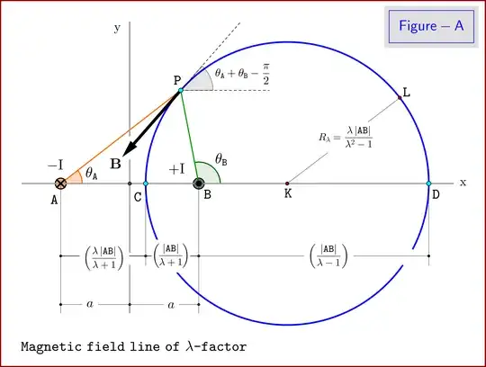
From equations \eqref{10} and \eqref{19} we have
\begin{equation}
\boxed{\:\:
\dfrac{\mr{PA}}{\mr{PB}}\e \lambda\,, \quad \lambda \bl\in \mathbb R^{\p}\:\:\vp}
\tl{20}
\end{equation}
that is
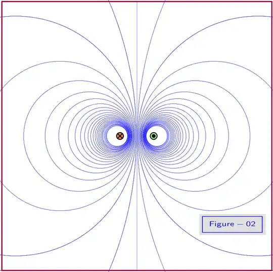
The magnetic field line corresponding to a positive factor $\:\lambda\:$ is the geometric locus of points $\:\mr P\:$ that see the edges of the straight segment $\:\mr{AB}\:$ with ratio $\:\lambda$. From geometry we know that these geometric loci are circles as shown in Figure-02.
In Figure-A details of the construction of a magnetic field line of $\lambda$-factor are shown.
Although we have proved that a magnetic field line is a perfect circle, we will give the parametric equations of this curve making use of equations \eqref{04} repeated here for convenience
\begin{align}
x_\theta\plr{\theta_{\mr A}} & \e \dfrac{\tan\theta_{\mr B}\p\tan\theta_{\mr A}}{\tan\theta_{\mr B}\m\tan\theta_{\mr A}}\, a
\tl{21a}\\
y_\theta\plr{\theta_{\mr A}} & \e \dfrac{2\tan\theta_{\mr B} \tan\theta_{\mr A}}{\tan\theta_{\mr B} \m \tan\theta_{\mr A}}\, a
\tl{21b}
\end{align}
In above equation we replace the angle $\:\theta_{\mr B}\:$ as function of the angle $\:\theta_{\mr A}\:$ according to \eqref{19}
\begin{equation}
\theta_{\mr B} \e \arcsin\plr{\lambda\sin\theta_{\mr A}}
\tl{22}
\end{equation}
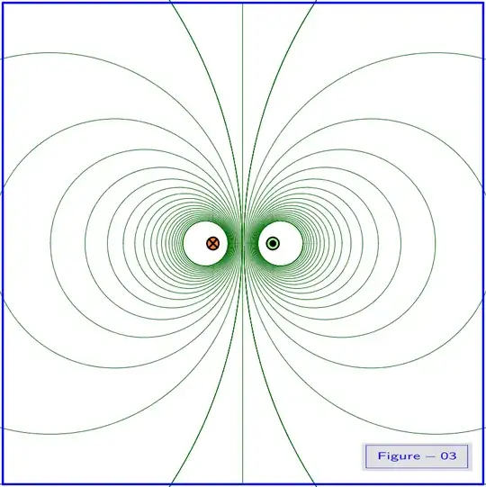
so the $\:{\color{red}{\bl{\theta_{\mr A}}}}\m$parametric equations for the magnetic field line of $\:{\color{blue}{\bl\lambda}}\m$factor are
\begin{align}
x_{\color{blue}{\bl\lambda}}\plr{{\color{red}{\bl{\theta_{\mr A}}}}} & \e \dfrac{\tan\blr{\arcsin\plr{{\color{blue}{\bl\lambda}}\sin{\color{red}{\bl{\theta_{\mr A}}}}}\vp}\p\tan{\color{red}{\bl{\theta_{\mr A}}}}}{\tan\blr{\arcsin\plr{{\color{blue}{\bl\lambda}}\sin{\color{red}{\bl{\theta_{\mr A}}}}}\vp}\m\tan{\color{red}{\bl{\theta_{\mr A}}}}}\, a
\tl{23a}\\
y_{\color{blue}{\bl\lambda}}\plr{{\color{red}{\bl{\theta_{\mr A}}}}} & \e \dfrac{2\tan\blr{\arcsin\plr{{\color{blue}{\bl\lambda}}\sin{\color{red}{\bl{\theta_{\mr A}}}}}\vp}\tan{\color{red}{\bl{\theta_{\mr A}}}}}{\tan\blr{\arcsin\plr{{\color{blue}{\bl\lambda}}\sin{\color{red}{\bl{\theta_{\mr A}}}}}\vp}\m\tan{\color{red}{\bl{\theta_{\mr A}}}}}\, a
\tl{23b}\\
\vp{\color{red}{\bl{\theta_{\mr A}}}} & \bl\in \plr{0,\pi}\,, \qquad {\color{blue}{\bl\lambda}}\bl\in \plr{0,\p\infty}
\tl{23c}
\end{align}
Using above parametric equations the magnetic field lines for various values of $\:{\color{blue}{\bl\lambda}}\:$ are shown in Figure-03. This Figure is precisely identical to Figure-02.