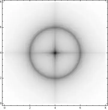
This probably isn't exactly what you're looking for, but if you're looking for the time-independent bound states of a system, the Fourier grid Hamiltonian method may be applicable. Here is an application of it to the following strange-looking potential well:
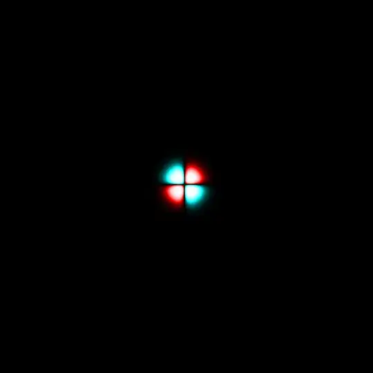
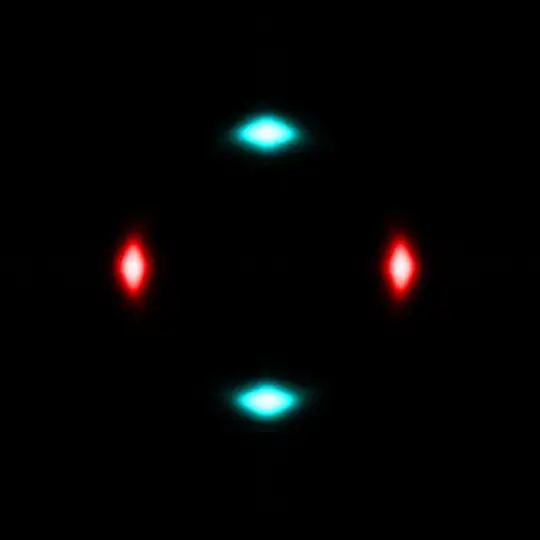
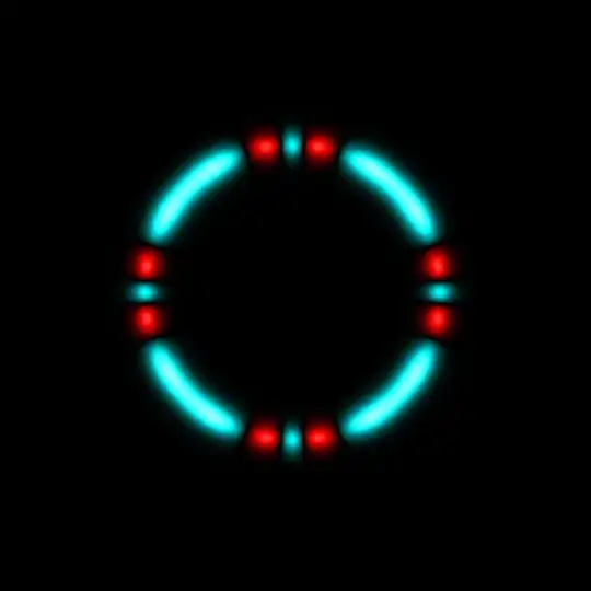
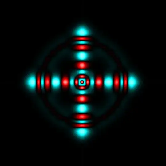
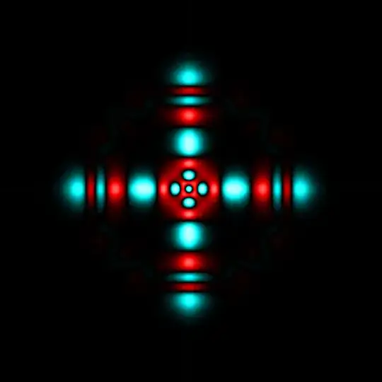
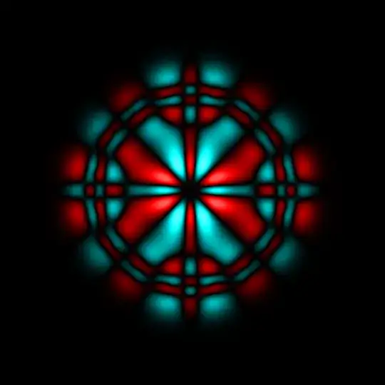
Here are a few low-energy bound states:
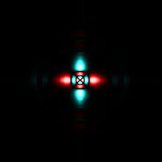
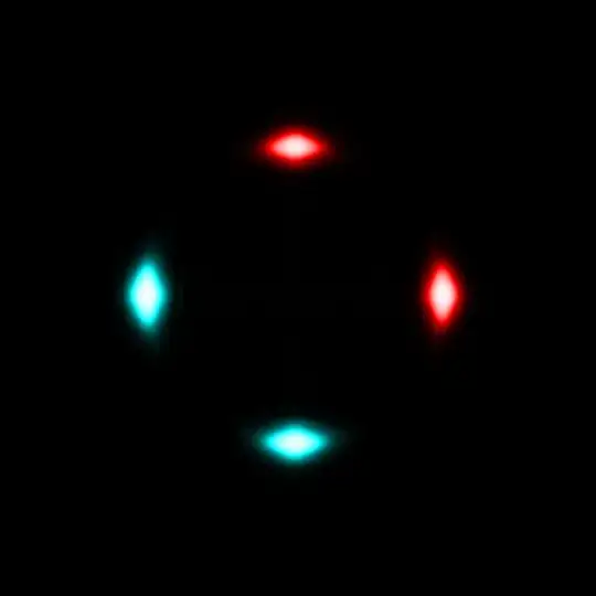
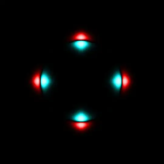
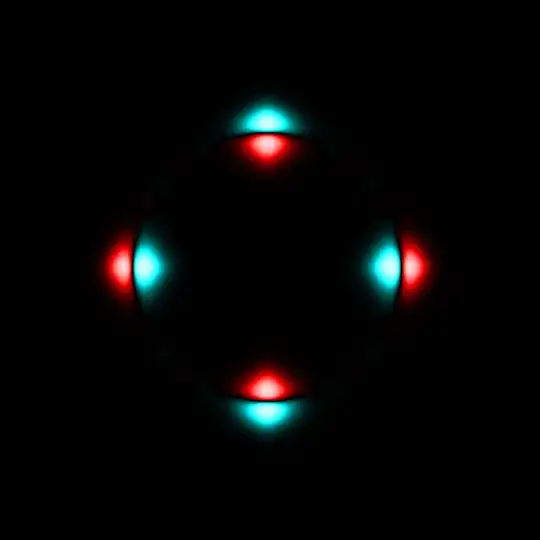
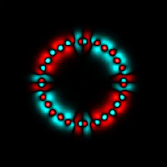
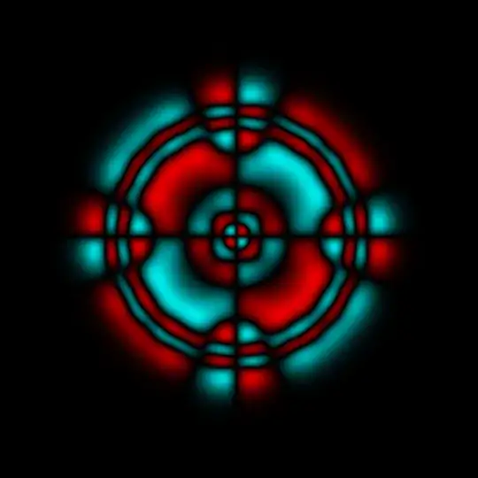
And here are some of the high-energy states:
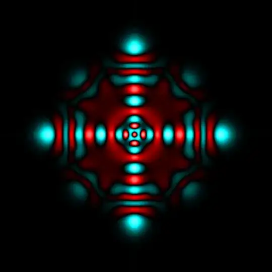
I used a fairly symmetric-looking potential surface, but you can do arbitrary shapes or squiggly lines if you really wanted to.
Here is Mathematica code used to draw the potential and compute the bound states. Beware that in 2D, just using 81 grid points in each dimension means that you have to diagonalize a $6561\times 6561$ matrix, which can take several minutes. The following defines the spatial axes and constructs the kinetic energy matrix:
$HistoryLength = 0;
hue = Compile[{{z, _Complex}}, {(1.0 Arg[-z] + \[Pi])/(2 \[Pi]),
    Exp[1 - Max[Abs[z], 1]], Min[Abs[z], 1]},
   CompilationTarget -> "C", RuntimeAttributes -> {Listable}];
vec[A_] := Flatten[Transpose[A, Reverse[Range[ArrayDepth[A]]]]];
nx1 = 8;
np1 = 8;
nn1 = nx1 np1;
L1 = 8;
\[CapitalDelta]x1 = L1/nx1;
\[CapitalDelta]p1 = 2 \[Pi]/\[CapitalDelta]x1;
\[Alpha]1 = \[CapitalDelta]p1/(2 \[CapitalDelta]x1);
pMax1 = \[CapitalDelta]p1 np1/2;
axis1 = (Range[nn1] - 1/2) L1/nn1;
TRow1 = If[EvenQ[nn1],
   1/2 Append[
     Table[(2.0 pMax1^2)/nn1^2 (-1)^j/Sin[\[Pi] j/nn1]^2, {j,
       nn1 - 1}], pMax1^2/3 (1 + 2.0/nn1^2)],
   1/2 Append[
     Table[(2.0 pMax1^2)/nn1^2 ((-1)^j Cos[\[Pi] j/nn1])/
       Sin[\[Pi] j/nn1]^2, {j, nn1 - 1}],
     pMax1^2/3 (1 + 1.0/nn1^2)]];
T1 = MapIndexed[RotateRight, ConstantArray[TRow1, nn1]];
nx2 = 8;
np2 = 8;
nn2 = nx2 np2;
L2 = 8;
\[CapitalDelta]x2 = L2/nx2;
\[CapitalDelta]p2 = 2 \[Pi]/\[CapitalDelta]x2;
\[Alpha]2 = \[CapitalDelta]p2/(2 \[CapitalDelta]x2);
pMax2 = \[CapitalDelta]p2 np2/2;
axis2 = (Range[nn2] - 1/2) L2/nn2;
TRow2 = If[EvenQ[nn2],
   1/2 Append[
     Table[(2.0 pMax2^2)/nn2^2 (-1)^j/Sin[\[Pi] j/nn2]^2, {j,
       nn2 - 1}], pMax2^2/3 (1 + 2.0/nn2^2)],
   1/2 Append[
     Table[(2.0 pMax2^2)/nn2^2 ((-1)^j Cos[\[Pi] j/nn2])/
       Sin[\[Pi] j/nn2]^2, {j, nn2 - 1}],
     pMax2^2/3 (1 + 1.0/nn2^2)]];
T2 = MapIndexed[RotateRight, ConstantArray[TRow2, nn2]];
The following allows you to enter a potential surface and plot it (the code below takes Potential to be the strange crosshair-shaped surface I showed at the beginning, but it can be changed to other shapes):
\[Delta] = 0.3;
Potential[x1_,
   x2_] := -600 \[Delta]/(Sqrt[(x1 - L1/2)^2] + \[Delta]) \[Delta]/(
    Sqrt[(x2 - L2/2)^2] + \[Delta]) -
   300 \[Delta]/(
    Abs[Sqrt[(x1 - L1/2)^2 + (x2 - L2/2)^2] - 2] + \[Delta]);
Hamiltonian[x1_, p1_, x2_, p2_] := (p1^2 + p2^2)/2 + Potential[x1, x2];
DensityPlot[Hamiltonian[x1, 0, x2, 0], {x1, 0, L1}, {x2, 0, L2},
 PlotRange -> All, PlotPoints -> 90, ColorFunction -> GrayLevel]
The following constructs the Hamiltonian and diagonalizes it:
V = DiagonalMatrix[
   vec[Table[
     Potential[axis1[[k1]], axis2[[k2]]], {k1, nn1}, {k2, nn2}]]];
T = KroneckerProduct[T2, IdentityMatrix[nn1]] +
   KroneckerProduct[IdentityMatrix[nn2], T1];
H = T + V;
{\[Lambda], \[CapitalLambda]} = {#1[[Ordering[#1]]], \
#2[[Ordering[#1]]]} & @@ Eigensystem[H];
And the following plots the bound states:
mat[v_] := Partition[v, nn1]\[Transpose];
interp[m_] :=
  8 InverseFourier[
    RotateLeft[
     PadRight[RotateRight[Fourier[m], Floor[Dimensions[m]/2]],
      8 Dimensions[m]], Floor[Dimensions[m]/2]]];
Manipulate[{\[Lambda][[k]],
  If[Abs[\[Lambda][[k - 1]] - \[Lambda][[k]]] <= 0.01 ||
    Abs[\[Lambda][[k + 1]] - \[Lambda][[k]]] <= 0.01, "Mixed",
   "Pure"],
  Image[hue[20 interp[mat[\[CapitalLambda][[k]]]]], ColorSpace -> Hue,
    Magnification -> 1]}, {k, 1, 500, 1}]
Unfortunately I don't exactly remember what physical units system the code uses, but I do remember that I wrote it partially based on David Tannor's exposition of the FGH method as outlined in his book Quantum Mechanics: A Time-Dependent Perspective.