The best rule of thumb I can give is that if the zeroth-order spectrum has a continuum part (like it always does in atomic/molecular physics), you should include it in your calculations because it is almost certainly important. The good news is that $-$ as shown below $-$ this contribution is often trivial to include; in many practical cases, we calculate it without even realizing!
A simple example on the importance of continuum states
Let us say that you want to expand $\exp(-r/2)$ in the basis of hydrogenic functions. Due to symmetry, only the $l=0$ part of the basis is needed:
$$
\exp\left(-\frac{r}{2}\right)=\sum_{n=1}^\infty C_n \, R_{n0}(r)+\int_0^\infty\mathrm{d}\varepsilon \, C_\varepsilon \, R_{\epsilon0}(r) \ ,
$$
where
$$
R_{n0}(r)=\frac{2}{n^{5/2}}\exp\left(-\frac{r}{n}\right)L_{n-1}^{(1)}\left(\frac{2r}{n}\right) \ ,
$$
and
$$
R_{\varepsilon0}(r)=\sqrt{\frac{2k}{\pi}}\exp\left(\frac{\pi}{2k}\right)\left|\Gamma\left(1+\frac{i}{k}\right)\right|\exp(-ikr) \, _1F_1\left(1+\frac{i}{k},2,2ikr\right) \,
$$
with $k=\sqrt{2\varepsilon}$. The coefficients are of course computed as
$$
C_n=\int_0^\infty\mathrm{d}r \, r^2 \, R_{n0}(r)\exp\left(-\frac{r}{2}\right) \ \ , \ \ C_\varepsilon=\int_0^\infty\mathrm{d}r \, r^2 \, R_{\varepsilon0}(r)\exp\left(-\frac{r}{2}\right) \ .
$$
It is not hard to check that by using only the discrete part of the basis, the expansion converges to the wrong function:
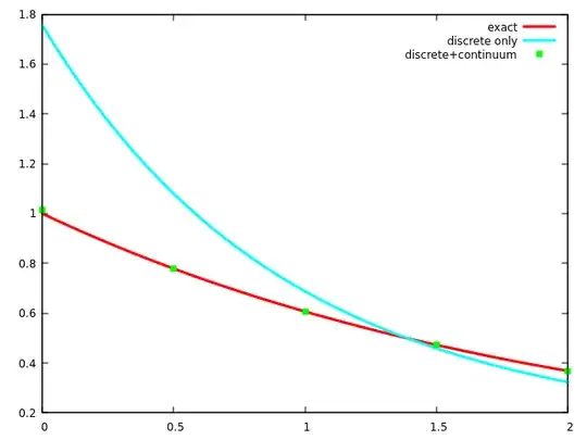
Such a simple function, yet it cannot be properly approximated without the continuum. This already shows that the problem is more general than perturbation theory. Trying to approximately turn the Schrödinger equation into a finite matrix eigenvalue equation by expanding the wave function over the discrete part of some known eigenbasis is in general a doomed attempt: the solution of the matrix problem will usually not converge to the exact solution.
Including scattering state contributions easily
Of course, in the basis of rescaled hydrogenic functions, the expansion of the above function is trivial: $\exp(-r/2)\sim R_{10}(r/2)$, displaying (not surprisingly) that what looks very complicated in one basis might be simple in another one.
This is exactly why variational optimization is such a powerful technique to accurately solve the Schrödinger equation even in a heavily truncated expansion: a compact linear combination of a "few" functions with parameters tweaked in order to minimize some functional (such as a Hamiltonian expectation value) is equivalent to a highly non-trivial expansion in another basis heavily involving continuum contributions (that basis spanned by e.g. the eigenfunctions of a simpler Hamiltonian); see e.g. Shull & Löwdin, J. Chem. Phys. 23 1362 (1955) for perhaps the first serious study on this issue. This is the rationale behind those extremely accurate variational computations for small few-electron systems, and this is how in practice accurate perturbative calculations are done with the Hylleraas functional (mentioned in my older answer).
But at this point you might wonder how anything can be calculated with a reasonable accuracy in e.g. quantum chemistry, where all computations are performed with fixed (pre-optimized) Gaussian basis functions, and no one starts tweaking those Gaussian parameters when dealing with specific problems. It turns out that continuum contributions are there even in a finite matrix representation without further optimization! As a (hopefully useful) example, let us see how the second-order PT energy and the "exact" clamped-nucleus ground state energy of helium is calculated in a quantum chemistry approach. The problem is first attacked with hydrogen-like orbitals, then with Hartree-Fock orbitals.
1. Ground state of helium: hydrogenic orbitals
I use the so-called aug-cc-pV5Z basis, one of the standardized Gaussian basis sets of electronic structure theory, containing $N_\text{b}=62$ basis functions in total (I had to remove basis functions of $G$ symmetry for technical reasons, but this is not important). Diagonalizing the matrix
$$
h_{\mu\nu}=\left\langle\chi_\mu\left|-\frac{1}{2}\nabla^2-\frac{Z}{r}\right|\chi_\nu\right\rangle
$$
gives us the orbitals of the hydrogen-like system (with $Z=2$) as linear combinations of Gaussians:
$$
\phi_p(\vec{r})=\sum_{\mu=1}^{N_\text{b}}c_{\mu p}\chi_\mu(\vec{r}) \ ,
$$
and the following orbital energies (multiplicities in parentheses):
$$
\begin{aligned}
\varepsilon_{1s}&\approx-1.99994 \\
\varepsilon_{2s}&\approx-0.49845 \\
\varepsilon_{2p}&\approx-0.49675 \ (\times3) \\
\varepsilon_{3s}&\approx-0.15930 \\
\varepsilon_1&\approx{\color{white}-}0.08937 \ (\times5) \\
\varepsilon_2&\approx{\color{white}-}0.13423 \ (\times3) \\
\varepsilon_3&\approx{\color{white}-}1.00968 \\
\varepsilon_4&\approx{\color{white}-}1.29781 \ (\times7) \\
\varepsilon_5&\approx{\color{white}-}2.10812 \ (\times5) \\
\varepsilon_6&\approx{\color{white}-}2.33411 \ (\times3) \\
\varepsilon_7&\approx{\color{white}-}5.92634 \\
\varepsilon_8&\approx{\color{white}-}6.54658 \ (\times7) \\
\varepsilon_9&\approx{\color{white}-}8.71016 \ (\times5) \\
\varepsilon_{10}&\approx{\color{white}-}9.54698 \ (\times3) \\
\varepsilon_{11}&\approx \, \, 24.48918 \ (\times7) \\
\varepsilon_{12}&\approx \, \, 29.95862 \ (\times5) \\
\varepsilon_{13}&\approx \, \, 30.94743 \\
\varepsilon_{14}&\approx \, \, 32.49725 \ (\times3) \ .
\end{aligned}
$$
The bound state energies follow $\varepsilon_{n}=-Z^2/(2n^2)$, the small difference between the $2s$ and $2p$ levels being a basis set error. Note that based on the signs of the energies, only 6 hydrogenic orbitals represent bound electrons of the total 62; all the others have positive energies, so they necessarily represent the continuum of scattering states despite the fact that all of them are expanded over Gaussians localized at the nucleus. The situation is somewhat similar to the case of Wannier states where highly delocalized functions are combined to obtain localized ones: here, these positive energy linear combinations of Gaussians can be thought of as localized combinations of the exact hydrogenic scattering states, spanning approximately the same space.
The ground state energy of helium up to second order is
$$
{\cal{E}}=\underbrace{2\varepsilon_{1s}+\left\langle\phi_{1s}\phi_{1s}\left|W\right|\phi_{1s}\phi_{1s}\right\rangle}_{={\cal{E}}^{(0)}+{\cal{E}}^{(1)}}+{\cal{E}}^{(2)} \ ,
$$
where the electron-electron interaction $W=1/r_{12}$ is the perturbation, and
$$
{\cal{E}}^{(2)}=
-2\sum_{a\neq1s}\frac{\left|\left\langle\phi_{1s}\phi_{1s}\left|W\right|\phi_{a}\phi_{1s}\right\rangle\right|^2}{\epsilon_a-\varepsilon_{1s}}-\sum_{a,b\neq1s}\frac{\left|\left\langle\phi_{1s}\phi_{1s}\left|W\right|\phi_{a}\phi_{b}\right\rangle\right|^2}{\epsilon_a+\epsilon_b-2\varepsilon_{1s}} \ .
$$
The $a,b$ sums represent summation/integration over bound/scattering states, which are replaced by summations over the orbitals in the finite matrix representation. The following table shows results obtained in the finite matrix representation compared to reference values:
\begin{array}{l|c|c}
& \text{Gaussian basis} & \text{reference} \\
\hline
{\cal{E}}^{(0)}+{\cal{E}}^{(1)} & -2.7500 & -2.7500 \\
{\cal{E}}^{(2)} & -0.1563 & -0.1577 \\
{\cal{E}}^{(2)}_\text{bound only} & -0.0692 & -0.0631 \\
{\cal{E}}^{(0)}+{\cal{E}}^{(1)}+{\cal{E}}^{(2)} & -2.9063 & -2.9077 \\
{\cal{E}}_{\text{exact(CCSD)}} & -2.9031 & -2.9037 \\
{\cal{E}}_{\text{exact(CCSD), bound only}} & -2.8541 & \text{n.a.}
\end{array}
In the "bound only" calculations, the sums were restricted to the 6 bound state orbitals; the results agree well with the reference values in each case (see the older answer for the reference values, computed with the exact hydrogenic eigenstates or variationally). We see that roughly 50-60% of the second-order energy and one-third of ${\cal{E}}_{\text{exact(CCSD)}}-[{\cal{E}}^{(0)}+{\cal{E}}^{(1)}]$ is attributed to the continuum.
2. Ground state of helium: Hartree-Fock orbitals
We saw that hydrogenic continuum states of the Coulomb potential are important contributors to the energy of helium. When working with HF orbitals instead, an even stronger, surprising statement can be made: the HF equation has only a single bound eigenstate (the lowest energy, $1s$), and all other eigenstates are scattering states! This means that the Slater determinant representing the ground state (doubly occupied by the $1s$ orbital) is the only genuine bound state in the two-electron determinant basis, all other states have at least one electron in a HF scattering state; restricting ourselves to purely bound states would mean that the ${\cal{E}}_\text{corr}={\cal{E}}_\text{exact}-{\cal{E}}_\text{HF}$ correlation energy vanishes, and we could not move beyond the HF approximation.
To see how this is possible, let us first investigate the exact HF equation without any Gaussian expansion. The equation reads
$$
\left[-\frac{1}{2}\nabla^2-\frac{Z}{r}+U_{\text{HF}}\right]\phi_p(\vec{r})=\varepsilon_p \, \phi_p(\vec{r}) \ ,
$$
where
$$
U_{\text{HF}} \, \phi_p(\vec{r})=2\int\mathrm{d}^3r'\frac{|\phi_{1s}(\vec{r}{}')|^2}{|\vec{r}-\vec{r}{}'|} \, \phi_p(\vec{r})-\int\mathrm{d}^3r'\frac{\phi^*_{1s}(\vec{r}{}')\phi_p(\vec{r}{}')}{|\vec{r}-\vec{r}{}'|} \, \phi_{1s}(\vec{r}) \ .
$$
Introducing $\phi_p(\vec{r})=(1/r)\psi_{\nu l}(r)Y_{lm}(\theta,\phi)$ and using the Laplace expansion to process the angular part, we get
$$
\left[-\frac{1}{2}\frac{\mathrm{d}^2}{\mathrm{d}r^2}-\frac{Z}{r}+\int_0^\infty\mathrm{d}r'\frac{\psi^2_{1s}(r')}{r_>}\right]\psi_{1s}(r)=\varepsilon_{1s} \, \psi_{1s}(r)
$$
for the ground state, and
$$
\begin{aligned}
\left[-\frac{1}{2}\frac{\mathrm{d}^2}{\mathrm{d}r^2}+\frac{l(l+1)}{2r^2}-\frac{Z}{r}+2\int_0^\infty\mathrm{d}r'\frac{\psi^2_{1s}(r')}{r_>}\right]\psi_{\nu l}(r)& \\
-\frac{1}{2l+1}\int_0^\infty\mathrm{d}r'\frac{r_<^l}{r^{l+1}_>}\psi_{1s}(r')\psi_{\nu l}(r') \, \psi_{1s}(r)&=\varepsilon_{\nu l} \, \psi_{\nu l}(r)
\end{aligned}
$$
for the excited states (with $\nu l \neq1s$). Note that $\psi_{1s}$ is determined by the first equation, and used as an input in the second one. For large $r$, we have
$$
-\frac{Z}{r}+\int_0^\infty\mathrm{d}r'\frac{\psi^2_{1s}(r')}{r_>}\sim-\frac{Z-1}{r} \ ,
$$
$$
-\frac{Z}{r}+2\int_0^\infty\mathrm{d}r'\frac{\psi^2_{1s}(r')}{r_>}\sim-\frac{Z-2}{r} \ ,
$$
while the exchange term becomes exponentially small.
The electron in the ground state sees a screened nuclear charge $Z-1$ for large distances due to the partial shielding of the other electron. A (hypothetical) electron in an excited state sees $Z-2$ for large distances due to the screening by both occupied electrons, so for the electrically neutral case of $Z=2$, the potential falls to zero very (exponentially) fast, and is not expected to be able to support bound states. This argument is similar to the one about the non-existence of excited states in H$^{-}$, and is readily generalized to the HF solutions of an electrically neutral $N$-electron atom (with only the first $\lceil N/2\rceil$ spatial orbitals being bound eigenstates). This is by no means a rigorous proof that atoms never have bound excited HF orbitals, but for a rule of thumb, this is as good as it gets. This argument is from Kelly, Phys. Rev. 131 684 (1963), where it was shown to hold for the beryllium atom (and for oxygen, in later work).
As an alternative argument, note that the potential decays exponentially fast for neutral atoms, and it is no more singular than $1/r$ for small distances. We can then apply Levinson's theorem, which states that the number of bound states the central potential can support is equal to the number of times the wave function changes sign in a zero-energy scattering. Therefore, the number of bound states for a given $l$ can be guessed by solving the excited state HF equation for $\varepsilon_l=0$. Since the potential vanishes so quickly for large $r$, the wave function can evidently change sign only a finite number of times before "flying off":
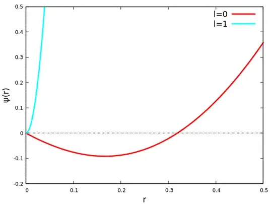
Quantitatively speaking, the plot might not be very accurate, because the iterative solution of the integro-differential equation is not stable, but the qualitative information is correct. There is one sign change in $\psi(r)$ for $l=0$ and none for $l=1$ (and generally for $l>0$), showing that the only bound state here is the $1s$. In the above Kelly paper about beryllium, two sign changes were found for $l=0$ and similarly none for $l>0$, implying that $1s$ and $2s$ are the only bound HF orbitals.
The same conclusions are drawn if the HF equation is solved in the finite matrix representation with the aug-cc-pV5Z Gaussians. Only one negative-energy (therefore bound) orbital is found (with the correct value $\varepsilon_{1s}\approx-0.9180$), all other states have positive energies. The energy up to second order is ${\cal{E}}={\cal{E}}_{\text{HF}}+{\cal{E}}^{(2)}$, where ${\cal{E}}^{(2)}$ takes a simpler form when evaluated with HF orbitals:
$$
{\cal{E}}^{(2)}=
-\sum_{a,b\neq1s}\frac{\left|\left\langle\phi_{1s}\phi_{1s}\left|W\right|\phi_{a}\phi_{b}\right\rangle\right|^2}{\epsilon_a+\epsilon_b-2\varepsilon_{1s}} \ .
$$
The numerical results are the following:
\begin{array}{l|c|c}
& \text{Gaussian basis} & \text{reference} \\
\hline
{\cal{E}}_{\text{HF}} & -2.8616 & -2.8617 \\
{\cal{E}}^{(2)} & -0.0386 & -0.0374 \\
{\cal{E}}_\text{HF}+{\cal{E}}^{(2)} & -2.9002 & -2.8991 \\
{\cal{E}}_{\text{exact(CCSD)}} & -2.9031 & -2.9037
\end{array}
The main point here is that without the continuum, there would be no correction to the HF energy. Note that the same exact(CCSD) energy is found as before, with the hydrogenic orbitals (the one-particle bases spanned by the hydrogenic and HF orbitals are connected by a unitary transformation, under which perturbative energy corrections are not invariant, but of course the exact energy is).
3. Conclusion
These numbers all confirm that the contribution of continuum states is there in the matrix representation of the problem, and when summing over the orbitals, we usually include it without even thinking about it.
In a sense, this helium example is too simple, since the parameters of the standardized Gaussian basis were most likely optimized for the atomic ground state energy. But the point is that the same conclusions would hold for a general molecular calculation where the total Gaussian basis consists of a sum of separate atomic basis sets. In polyatomic cases, distinguishing between genuine bound states and "wannierized" scattering states might be difficult (the simple sign criterium that was used above generally does not work), but it is enough to know that the continuum is there in the background, and its effect is included in the results.

