15

Sorry for the provocative title. There's probably something wrong with my reasoning, and maybe someone will bother to point it out.

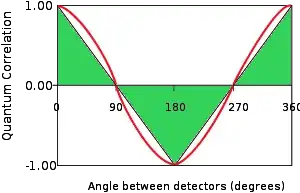
I did not understand Bell's Theorem, so I looked for easy explanations. I found one that looked very intuitive. They set up something like light polarization, but simpler. They explained that given "reasonable" assumptions, you must predict a linear change in correlation with the angle between detectors. The difference between 90 degrees and 91 degrees must be the same as the difference between 45 degrees and 46 degrees. But in fact it doesn't work that way, so the "reasonable" assumptions must be wrong.

picture

That made sense. Then I found a coherent explanation with equations.

This elegantly describes what properties a "reasonable" set of assumptions must have, and describes an experiment that no "reasonable" assumptions can give a correlation better than .75 for. The claim is that QM predicts more than .75, and experiment is consistent with QM and not with "reasonable" assumptions.

Background

We assume there is some system state $\lambda$. There are two detectors $x, y$ which have outcomes $a, b$. Each outcome can only be 0 or 1.

The experimenters measure $p(ab|xy)$. They don't know $\lambda$, but they have estimated probabilities for some states that $\lambda$ might be in, so what they're really measuring is

$\underset{\lambda}{\sum}{p(ab|xy\lambda) p(\lambda|xy)}$

Further assumptions:

  1. $\lambda$ is not correlated with $x$ or $y$.

$$p(\lambda|xy)=p(\lambda)$$

Given that,

$$p(ab|xy) = \underset{\lambda}{\sum}{p(ab|xy\lambda) p(\lambda)}$$

  1. $x, y$ and $\lambda$ are enough to completely determine $a, b$

$$p(ab|xy) \in \{0, 1\}$$

That results in

$$p(ab|xy) = \underset{\lambda}{\sum}{p(a|xy\lambda) p(b|xy\lambda) p(\lambda)}$$

  1. $x$ does not influence $b$ and $y$ does not influence $a$.

$$p(a|xy\lambda)=p(a|x\lambda)$$

$$p(b|xy\lambda)=p(b|y\lambda)$$

So

$$p(ab|xy) = \underset{\lambda}{\sum}{p(a|x\lambda) p(b|y\lambda) p(\lambda)}$$

And from there he goes on to demonstrate the thing that can't correlate better than .75. It's very clear, I highly recommend it. He expands on that in a couple of later posts.

My efforts

Given this understanding, I tried an example, polarized light. Given a photon with linear polarization angle 0 and a polarizer with polarization angle $\theta$, that has two outcomes 0 and 1, the probability that the photon has outcome 0 is $\cos^2{\theta}$. I ran various simulations using Glowscript, a simple graphics programming system that often lets you see your mistakes in the way the pictures come out.

For every x and y between 0 and $2\pi$, I integrated over $\theta$ to get the probability that the outcomes a and b were the same.

If a and b were independent, then

$$p(a|xy\theta)=cos^2(x-\theta)$$

$$p(b|xy\theta)=cos^2(y-\theta)$$

$$p(ab|xy\theta)=cos^2(x-\theta)cos^2(y-\theta)$$

But for entangled photons, a and b are not independent. The closer x and y are to each other, the more likely that a and b are the same, regardless of $\theta$. (Oops! For experimental entangled photons, they are opposite and not the same. I'm sure the results are equivalent, though.) The formula is

$$p(ab|xy\theta)=p(a|x\theta)p(b|axy\theta)=cos^2(x-\theta)cos^2(x-y)$$

Graphed out, this looks like

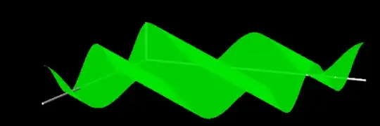
3D graph

(I went from 0 to $2\pi$ in each direction when it would have been enough to go from 0 to $\pi/2$, just in case my thinking was wrong and it would have made a difference.)

The correlation is the same whenever x-y is the same. This is just like the simple graph above except that one of the simplifications was to put the zeroes at 90 and 270 degrees, instead of at 45, 135, 225, and 315 degrees etc.

Again, the reason we get this result is that

$$p(ab|xy\theta)=p(a|x\theta)p(b|axy\theta)\neq p(a|x\lambda) p(b|y\lambda)$$

Photon polarization does not meet the criteria for Bell's inequality, which of course it must not or it could not be what it is. It looks to me like the assumptions behind Bell's inequality require that we must assume that the photons are not entangled. Assuming they are not entangled, of course we cannot get the same correlations we get when they are entangled.

Given that this is what it takes to get photon polarization to work, I didn't see why a deterministic system must fail. I quick found something that looked like it would work.

Each photon has three hidden variables. One is a polarization angle $\theta$ between 0 and 2 $\pi$.

Then there are two hidden variables $\rho$ and r between 0 and 1.

Same-entangled photons have all three of these variables the same.

To find whether a photon passes a filter with angle $\lambda$, calculate $\cos(\lambda-\theta)$. If $\rho, r$ are inside the square defined by (0,0) $(\cos(\lambda-\theta),\cos(\lambda-\theta))$ then it passes the filter.

Then set $\theta$ to $\lambda$. Multiply $\rho$ and r by 7 and discard any part of the results that are bigger than 1, to get their new values.

Question:

Since Bell's Theorem is correct, where did I go wrong?
Mauricio
  • 6,886
J Thomas
  • 3,146

5 Answers5

19

I'm really not a fan of the blog post you link, both due to the notation and to the specific focus on the somewhat opaque experiment described at the end. So I'll diverge from it to address your question. I'll start with some preliminary definitions and the statement/proof of the theorem. If you are already familiar with this, you can skip to the end of the answer.

Consider two detectors $X$ and $Y$ which return measurement values $x$ and $y$, respectively, where $x$ and $y$ may take the values $\pm 1$. Each detector has some additional settings $\alpha_X$ and $\alpha_Y$ which may be chosen freely and independently by the graduate students operating each detector. Finally, there is an additional "hidden variable" $\lambda$ which underlies the experiment and which may influence the experimental outcomes, but which is not influenced by the settings $\alpha_X$ and $\alpha_Y$ of the two detectors.

Under these conditions, we may define the correlation between the measurement results - which depend on the settings $\alpha_X$ and $\alpha_Y$ - as follows: $$C(\alpha_X,\alpha_Y) := \int \mathbb E_{\alpha_X,\alpha_Y}\big[xy|\lambda\big] \ p(\lambda) \mathrm d\lambda$$ where $$\mathbb E_{\alpha_X,\alpha_Y}[xy|\lambda]:= \sum_{x,y\in \{\pm 1\}} xy \ P^{XY}_{\alpha_X,\alpha_Y}(x,y|\lambda)$$ is the expected value of the product $xy$ given the settings $\alpha_X$ and $\alpha_Y$ and the hidden variable $\lambda$, $p(\lambda)$ is the PDF for the hidden variable, and $P^{XY}_{\alpha_X,\alpha_Y}$ is the joint PDF for the two experimental outcomes.

If we assume that the detector settings may be chosen independently in such a way that the measurement result at $X$ does not depend on the result at $Y$, then the joint PDF factorizes into $$P^{XY}_{\alpha_X,\alpha_Y}(x,y|\lambda) = P^X_{\alpha_X}(x|\lambda) P^Y_{\alpha_Y}(y|\lambda)$$ and so $$\mathbb E_{\alpha_X,\alpha_Y}\big[xy|\lambda\big] = \mathbb E_{\alpha_X}\big[x|\lambda\big] \mathbb E_{\alpha_Y}\big[y|\lambda\big]$$

If this is the case, then the CHSH inequality - the most common of a category of expressions which fall under the heading of "Bell inequalities" - says the following:

$$|C(a,b)-C(a,c)| + |C(d,b)+C(d,c)|\leq 2$$

for any choices of detector settings $a,b,c,d$.


Proof: The proof is very straightforward. Note that $$|C(a,b)-C(a,c)| = \left|\int \mathrm d\lambda\ p(\lambda) \mathbb E_a\big[x|\lambda\big] \big(\mathbb E_b\big[y|\lambda\big]-\mathbb E_c\big[y|\lambda\big]\big)\right|$$ $$\leq \int \mathrm d\lambda\ p(\lambda)\bigg|\mathbb E_b\big[y|\lambda\big]-\mathbb E_c\big[y|\lambda\big]\bigg|$$ Similarly, $$|C(d,b)+C(d,c)| \leq \int \mathrm d\lambda \ p(\lambda)\bigg|\mathbb E_b\big[y|\lambda\big] + \mathbb E_c\big[y|\lambda\big]\bigg|$$ It is an easily provable fact about real numbers $p,q\in[-1,1]$ that $|p-q|+|p+q|\leq 2$; the CHSH inequality follows immediately.


With those preliminaries out of the way, we can address your questions.

$\lambda$ is not correlated with $x$ or $y$. $p(\lambda|xy)=p(\lambda)$.

This notation suggests that $x$ and $y$ are random variables and that we're thinking about conditional probabilities. This is not the case - $x$ and $y$ (which I call $\alpha_X$ and $\alpha_Y$ in my notation) are the settings on the detectors, and are chosen freely and independently by our faithful graduate students. The assumption is that the PDF for our hidden variable $\lambda$ is not a function of what we choose for these settings.

As an example, we might imagine that the hidden variable turns out to be the temperature of the laboratory. In this context, the assumption is that the settings we choose for the dials on the experimental apparatuses do not influence the laboratory temperature.

After detector $x$ finds outcome $a$, now $\lambda$ is no longer independent. Different values for $\lambda$ would give different values for $a$, or else $\lambda$ wouldn't matter for predicting $a$. So if we know $x, a$ that gives us a clue about $\lambda$.

The fact that $p(\lambda)$ is not a function of $\alpha_X$ or $\alpha_Y$ does not imply that a given measurement gives us no clues about the possible values $\lambda$ might take. In particular, we are not claiming that the hidden variable $\lambda$ and the outcome of one of the detector measurements $x$ are uncorrelated for every choice of detector setting $\alpha_X$ - if we were, then Bayes' rule would tell us that $P^X_{\alpha_X}(x|\lambda) = P^X_{\alpha_X}(x)$, rendering the hidden variable pointless.

This is a weakness of the linked blog post, in my view. The word correlation implies (to me) that we're talking about two random variables. Instead, as mentioned above, our claim is that the PDF for $\lambda$ is not a function of the parameters $\alpha_X$ and $\alpha_Y$. In the context of our temperature example, the claim would be that the temperature of the lab is not influenced by the settings on the knobs of our detectors.

Is this how QM gets its correlation, or is it some other way that I have not noticed?

The general take-away from Bell's theorem is not that there is a limit on the correlation between our measurement results for any one choice of detector settings. Instead, the point is that if we are allowed to vary the detector settings locally and independently, then there is a limit on how the corresponding correlations may vary.

In other words, a violation of a Bell inequality means that our graduate students freely and independently changed their detector settings and that the subsequent correlations can not be accounted for by the assumption that a local hidden variable was determining their results.


I'll conclude by addressing your photon example. If we send an entangled pair of photons described by a spin-singlet state to detectors outfitted with polarizers whose orientation is defined by unit vectors $\vec a$ and $\vec b$ (these unit vectors are the "detector settings" described above) and whose outcomes are $+1$ for a detected photon and $-1$ for an undetected photon, then the correlation between our two detectors is given by $C(\vec a,\vec b)=-\vec a \cdot \vec b$ as per quantum mechanics. Plugging this into the CHSH inequality yields

$$|\vec a\cdot(\vec b-\vec c)| + |\vec d\cdot (\vec b+\vec c)| \leq 2$$

However, if we let $\vec a = \hat z$ and $\vec d = \hat x$ (so our first graduate student may turn her detector by $90^\circ$ at her leisure) and then let $\vec b = (\cos(\phi)\hat x+\sin(\phi)\hat z)/\sqrt{2}$ and $\vec c = (\sin(\phi)\hat x-\cos(\phi)\hat z)/\sqrt{2}$ (so our second graduate student may turn his detector by $90^\circ$ as well, but his orientations are offset from hers), then we find that the CHSH inequality becomes

$$2[\cos(\phi)+\sin(\phi)] \leq 2$$ which is clearly violated for $\phi \in (0,\pi/2)$.

As we see, the problem is not that the correlation between detectors is too high for any particular choice of orientations (indeed for appropriately chosen $\vec a$ and $\vec b$, we can clearly arrange for $C(\vec a,\vec b)=-\vec a \cdot \vec b$ to take any value in $[-1,1]$), but rather that upon independent variation of these orientations, we find correlations which violate the CHSH inequality and therefore are not consistent with our assumptions regarding local hidden variables.

Albatross
  • 72,909
9

Bell's Theorem is fine mathematics, but the universe is under no obligation to agree with it. Mathematics is not physics.

The idea that we use to capture the actual phenomenon is that once you have measured one photon in the pair, you've forced the other photon's state to conform to the measurement. But it doesn't possess that state before your first measurement: if it did, Bell's Theorem would apply.

John Doty
  • 22,119
4

In the quantum mechanical case $\lambda$ is fixed; in particular it is not correlated with $a,b,x,y$. It is simply the quantum state $\psi$.

In the simplest version of Bell's theorem, the assumption that quantum mechanics violates is that of determinism, i.e. that $p(ab|xy) \in \{0,1\}$. This is already enough to demonstrate you won't be able to reproduce the quantum correlations with a deterministic model that is local, that is, such that $p(a|xy\lambda) = p(a|x\lambda)$ and $p(b|xy\lambda) = p(b|y\lambda)$.

One might think, though, that one can nevertheless reproduce the quantum correlations just by giving up on determinism, and still maintaining some sort of locality. That's why the nonlocal version of Bell's theorem is important: it shows that it is also impossible.

More specifically, it is not possible to violate a Bell inequality if $p(a|bxy\lambda) = p(a|x\lambda)$ and $p(b|axy\lambda) = p(b|y\lambda)$. That's the local causality assumption.

The interesting thing is that since we're not assuming determinism, this also applies to quantum mechanics, which implies that quantum mechanics must violate local causality in order to violate a Bell inequality, and indeed it does.

2

People tend to overcomplicate this. When we have two entangled polarised photons and pass them through polarising analysers (A and B) the correlation probability is given by $$p = \cos^2(\theta_A - \theta_B),$$

where $\theta_A$ and $\theta_B$ are the angles of the respective polarising analysers. If at the time of emission we secretly encode the position of polariser A in photon B as a hidden variable we could obtain the correct correlation, but the problem is that the angle of analyser A can be changed mid flight and somehow the hidden variable has to be updated to this new position to get the correct result. The problem for local hidden variable theories, is that if the polarising filters are spaced far apart and the photons arrive at their respective polarisers near enough simultaneously, there is not enough time for the position of polariser A to be communicated to photon B, if the communication is limited to the speed of light. It is not possible for photon B to know the new position of polariser A using only local information, so the local hidden variable theory fails and can not match actual measurements made in labs or the predictions of quantum theory.

A super-deterministic local hidden variable theory can replicate the results of quantum theory if by "super-deterministic" we mean the future is absolutely pre-determined and can be predicted with 100% accuracy. In this model if Anne is operating the A analyser, Anne has no free will and the position she will turn the analyser to, is inevitable and predictable. We could then encode photon B with information of the predicted position of analyser A at the future time when photon B arrives at analyser B.

KDP
  • 10,288
-5

The problem I have with Bell's Theorem is that its trying to use three vectors (lambda, x, and y here) to expand a two dimensional spin space. Any 3 vectors in that space will be linearly dependent, invalidating the independence assumption he's making and thus any steps afterwards.

Factoring out that relationship is the linear algebra equivalent of dividing by zero. After a move like that, you can "prove" that 2 = 1 a clear inconsistency. That's where I suspect the issue with his inequality comes from, and why both QM & experiment are correct while Bell's Theorem isn't.