Self-energy, 1PI, and tadpoles

Question

I'm having a hard time reconciling the following discrepancy:

Recall that in passing to the effective action via a Legendre transformation, we interpret the effective action $\Gamma[\phi_c]$ to be the generating functional of 1-particle irreducible Green's functions $\Gamma^{[n]}$. In particular, the 2-point function is the reciprocal of the connected Green's function,

$$\tilde \Gamma^{[2]}(p)=i\big(\tilde G^{[2]}(p)\big)^{-1}=p^2-m^2-\Sigma(p)$$

which is the dressed propagator.

But, the problem is this: in the spontaneously broken $\phi^4$ theory, the scalar meson (quantum fluctuations around the vacuum expectation value) receives self-energy corrections from three diagrams:

$-i\Sigma(p^2) = $ + +

Note that the last diagram (the tadpole) is not 1PI, but must be included (see e.g. Peskin & Schroeder p. 361). In the MS-bar renormalization scheme, the tadpole doesn't vanish.

If the tadpole graph is included in $\Sigma$, and hence in $\tilde{G}$ and $\tilde\Gamma$, then $\tilde\Gamma$ cannot be 1PI. If the tadpole is not included, then $\tilde G$ is not the inverse of the dressed propagator (that's strange, too). What's going on?

Answer 1

I'm going to give an explanation at the one loop level (which is the order of the diagrams given in the question).

At one loop, the effective action is given by $$ \Gamma[\phi]=S[\phi]+\frac{1}{2l}{\rm Tr}\log S^{(2)}[\phi],$$ where $S[\phi]$ is the classical (microscopic) action, $l$ is an ad hoc parameter introduced to count the loop order ($l$ is set to $1$ in the end), $S^{(n)}$ is the $n$th functional derivative with respect to $\phi$ and the trace is over momenta (and frequency if needed) as well as other indices (for the O(N) model, for example).

The physical value of the field $\bar\phi$ is defined such that $$\Gamma^{(1)}[\bar\phi]=0.$$ At the meanfield level ($O(l^0)$), $\bar\phi_0$ is the minimum of the classical action $S$, i.e. $$ S^{(1)}[\bar \phi_0]=0.$$ At one-loop, $\bar\phi=\bar\phi_0+\frac{1}{l}\bar\phi_1$ is such that $$S^{(1)}[\bar \phi]+\frac{1}{2l}{\rm Tr}\, S^{(3)}[\bar\phi].G_{c}[\bar\phi] =0,\;\;\;\;\;\;(1)$$ where $G_c[\phi]$ is the classical propagator, defined by $S^{(2)}[\phi].G_c[\phi]=1$. The dot corresponds to the matrix product (internal indices, momenta, etc.). The second term in $(1)$ corresponds to the tadpole diagram at one loop. Still to one-loop accuracy, $(1)$ is equivalent to $$ S^{(1)}[\bar \phi_0]+\frac{1}{l}\left(\bar\phi_1.\bar S^{(2)}+\frac{1}{2}{\rm Tr}\, \bar S^{(3)}.\bar G_{c}\right)=0,\;\;\;\;\;\;(2) $$ where $\bar S^{(2)}\equiv S^{(2)}[\bar\phi_0] $, etc. We thus find $$\bar \phi_1=-\frac{1}{2}\bar G_c.{\rm Tr}\,\bar S^{(3)}.\bar G_c. \;\;\;\;\;\;(3)$$

Let's now compute the inverse propagator $\Gamma^{(2)}$. At a meanfield level, we have the meanfield propagator defined above $G_c[\bar\phi_0]=\bar G_c$ which is the inverse of $S^{(2)}[\bar\phi_0]=\bar S^{(2)}$. This is what is usually called the bare propagator $G_0$ in field theory, and is generalized here to broken symmetry phases.

What is the inverse propagator at one-loop ? It is given by $$\Gamma^{(2)}[\bar\phi]=S^{(2)}[\bar\phi]+\frac{1}{2l}{\rm Tr}\, \bar S^{(4)}.\bar G_{c}-\frac{1}{2l}{\rm Tr}\, \bar S^{(3)}.\bar G_{c}. \bar S^{(3)}.\bar G_{c}, \;\;\;\;\;\;(4)$$ where we have already used the fact that the field can be set to $\bar\phi_0$ in the last two terms at one-loop accuracy. These two terms correspond to the first two diagrams in the OP's question. However, we are not done yet, and to be accurate at one-loop, we need to expand $S^{(2)}[\bar\phi]$ to order $1/l$, which gives $$\Gamma^{(2)}[\bar\phi]=\bar S^{(2)}+\frac{1}{l}\left(\bar S^{(3)}.\bar\phi_1+\frac{1}{2}{\rm Tr}\, \bar S^{(4)}.\bar G_{c}-\frac{1}{2}{\rm Tr}\, \bar S^{(3)}.\bar G_{c}. \bar S^{(3)}.\bar G_{c}\right). 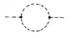\;\;\;\;\;\;$$ Using equation $(3)$, we find $$\bar S^{(3)}.\bar\phi_1= -\frac{1}{2}\bar S^{(3)}.\bar G_c.{\rm Tr}\,\bar S^{(3)}.\bar G_c,$$ which corresponds to the third diagram of the OP. This is how these non-1PI diagrams get generated in the ordered phase, and they correspond to the renormalization of the order parameter (due to the fluctuations) in the classical propagator.

Answer 2

(I came across this question while looking through the "unanswered" category. Not sure why a 9-month-old question appeared in the list, but there still seems to be a room for my contribution.)

The quantum effective action $\Gamma[\phi]$ generates 1PI diagrams, and a tree-level analysis on it amounts to a full analysis on the original action $S[\phi]$.

The sum of all 2-point 1PI diagrams is what contributes (in addition to $p^{2}-m^{2}$, which is also present in the original action) to the quadratic part of $\Gamma[\phi]$. If there were no term linear in $\phi$ in $\Gamma[\phi]$, this would be the self energy itself; however, if $\Gamma[\phi]$ contained a linear term, one has to do an additional tree-level calculation to obtain the self energy from $\Gamma[\phi]$.

As for Feynman diagrams in the original post, the first two contribute to $\Gamma[\phi]$, and the third one appears when calculating the self energy from $\Gamma[\phi]$.

Answer 3

1. The full 2-pt function is equal to the full connected 2-pt function plus tadpole contributions: $$\begin{align}\frac{\hbar}{i}G^{k \ell}~=~& \langle \phi^k\phi^{\ell} \rangle_{J=0} \cr ~=~&\langle \phi^k\phi^{\ell} \rangle^c_{J=0} +\langle \phi^k \rangle_{J=0} \langle \phi^{\ell} \rangle_{J=0}\cr ~=~&\frac{\hbar}{i} W_{c,2}^{k \ell} +W_{c,1}^k W_{c,1}^{\ell}. \end{align} , \tag{1}$$ cf. e.g. my Phys.SE answer here.

2. The self-energy $$ \Sigma~=~G_0^{-1}-G_c^{-1}\tag{2}$$ in general consists of connected diagrams with 2 amputated legs such that the 2 legs cannot be disconnected by cutting a single internal line, cf. e.g. my Phys.SE answer here.

   NB: Note in particular that the self-energy (2) may contain non-1PI diagrams with tadpoles, cf. OP's diagrams.

3. The quadratic term in the effective action $\Gamma[\phi_{\rm cl}]$ reads $$ \begin{align} (\Gamma_2)_{k\ell}~=~& ~-~(W^{-1}_{c,2})_{k\ell}\cr ~-~& W_{c,3}^{pqr}(W^{-1}_{c,2})_{pk}(W^{-1}_{c,2})_{q\ell}(W^{-1}_{c,2})_{rm}W^m_{c,1} \cr ~+~&{\cal O}((W_{c,1} )^2),\end{align}\tag{3}$$ cf. e.g. my Phys.SE answer here.

4. Conversely, the full/dressed connected propagator reads $$ \begin{align} G_c^{k\ell}~=~&W_{c,2}^{k\ell}\cr ~=~& ~-~(\Gamma^{-1}_2)^{k\ell}\cr ~-~& \Gamma_{3,pqr}(\Gamma^{-1}_2)^{pk}(\Gamma^{-1}_2)^{q\ell}(\Gamma^{-1}_2)^{rm}\Gamma_{1,m}\cr ~+~&{\cal O}((\Gamma_1)^2).\end{align}\tag{4}$$

5. $W_{c,2}^{k\ell}$ and $-(\Gamma_2)_{k\ell}$ become inverses of each other if $$\text{there are no tadpoles}\quad\Leftrightarrow\quad W_{c,1}^k~=~0\quad\Leftrightarrow\quad\Gamma_{1,k}~=~0,\tag{5}$$ cf. e.g. my Phys.SE answer here.

6. If there are no tadpoles, then OP's formulas simplify to $$ \Gamma_2 ~=~-W^{-1}_{c,2} ~=~-G_c^{-1}~=~-G_0^{-1} +\Sigma,\tag{6}$$ where the self-energy $\Sigma$ only contains 1PI diagrams.