Relativity (Planck)

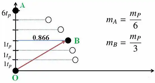
We take 2 particles A (v = 0 in 3D space) and B (v = 0.866c in 3D space). Both have a frequency = 6; 5t_p (5 increments to t_age) in the wave-state followed by 1t_p (1 increment to t_age) in the point-state (the point-state is represented by a black dot, diagram right).

The hyper-sphere expands radially at the speed of light. Both particles begin at the same space-port; defined as origin O. After 1 second, B will have traveled 299792458 * 0.866 = 259620km from A in 3-D space (the horizontal axis). However for both A and B the radial axis length is the same OA = OB.

As the surface of the hypersphere constitutes 3-D space, movement along this surface corresponds to distance travelled (in conventional terms). However as the hypersphere is expanding outward (time goes forward), the surface expands with it, and so the universe 4-axis co-ordinates would register as a space-time continuum. We would note that A has travelled 1 second in time but no distance in meters. B has travelled both in time and in space (259620km from stationary A).

In hypersphere co-ordinates, both A and B have travelled the same radial axis length; OA = OB. There is only 1 velocity and that is the velocity of expansion; radial axis OA will always equal OB. For 3D-surface-dwellers, there is a distinction between time and space because the 3D-surface-dweller has no means to register the hypersphere expansion as motion.

From the perspective of surface-dweller A (v = 0), B will have reached the point-state after 3 units of t_age (3 units of Planck time t_p) and so will have twice the (relativistic) mass of A. However the hypersphere expands radially from origin O, and so A will also have traveled the equivalent of 299792458m from O (radial axis OA = OB, v = c), and so from the perspective of the hypersphere, B can equally claim that A has traveled 259620km from B in 3-D space terms.

The time-line axis (axis of expansion) maps Planck time (1t_p) steps, note that only the particle point-state has defined co-ordinates, and so on this graph A can only have 6 possible time-line divisions (if including v = 0). As the minimum step is 1 unit of Planck time, this means that B can attain Planck mass (m_B = m_P/1) when at maximum velocity v_max (relative to the A time-line axis), but B can never attain the horizontal axis = velocity c because in the process at least 1 time step (1 unit of Planck time) is required, and so for particles v_max can never attain c. However a small particle such as an electron has more time-line divisions, and so can travel faster in 3-D space than can a larger particle (with a shorter wavelength).

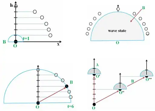
Depicted is particle B at some arbitrary universe time t = 1. B begins at origin O (top left) and is pulled (stretched) by the hyper-sphere (pilot wave) expansion in the wave-state (top right). At t = 6, B collapses back into the mass point state (bottom left) and now has new co-ordinates within the hypersphere, these co-ordinates becoming the new origin O’.

In hypersphere coordinates everything travels at, and only at, the speed of expansion = c, this is the origin of all motion, particles (and planets) do not have any inherent motion of their own, they are pulled along by this expansion as particles oscillate from (electric) wave-state to (mass) point-state ... ad-infinitum.

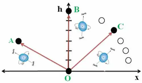
Particles are assigned an N-S spin axis around which particles can rotate (spin left and spin right). The co-ordinates of the point-state are determined by the orientation of the N-S axis. Of all the possible solutions, it is the particle N-S axis which determines where the point-state will next occur.

A, B and C begin together at O, if we can then change the N-S axis angle of A and C compared to B, then as the universe expands the A wave-state and the C wave-state will be stretched as with the B wave-state, but the point state co-ordinates of A (and C) will now reflect their new N-S axis angles of orientation.

A, B, C do not need to have an independent motion; they are being pulled by the universe expansion in different directions (relative to each other). We can thus simulate a transfer of physical momentum to a particle by simply changing the N-S axis. The radial hyper-sphere expansion does the rest.

In this example (diagram right), we continuously change the N-S axis of B (orange dot frequency f = 6) across all 11 options (f = 6 == 6 possible time-line divisions) after each point state.

A wave forms around the A (purple dot v = 0) time-line axis with a period ${\displaystyle 4(4f^{2}-f)}$ measured in time units;

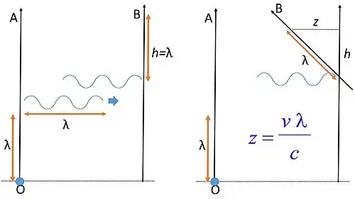
Information between particles is exchanged by photons. Photons do not have a mass point-state, only a wave-state, and so have no means to travel the radial expansion axis, instead they travel laterally across the hyper-sphere (they are `time-stamped', a photon reaching us from the sun is 8 minutes old).

The period required for particles to emit and to absorb photons is proportional to photon wavelength as illustrated in the diagram (right), ${\displaystyle A}$ (v = 0, left column) emits a photon (wavelength ${\displaystyle \lambda }$) towards ${\displaystyle B}$ (right column). The time taken (h) by ${\displaystyle B}$ to absorb the photon depends on the motion of ${\displaystyle B}$ relative to ${\displaystyle A}$. The Doppler shift;

${\displaystyle v_{observed}=v_{source}.{\frac {\sqrt {1-{\frac {v^{2}}{c^{2}}}}}{1-{\frac {v}{c}}}}=v_{source}.{\frac {h}{\lambda -z}}}$

Photons cannot travel the radial expansion axis, and as the information between particles is exchanged via the electromagnetic spectrum, ABC will measure only the horizontal AB, BC and AC (x-y-z) co-ordinates, thus defining for the 3 observers (A, B and C) a relativistic 3-D space. Relativity formulas translate between the 4-axis hyper-sphere and the 3-D space co-ordinate systems.

All particles simultaneously in the point-state at any unit of t_age form orbital pairs with each other ^[3]. These orbital pairs then rotate by a specific angle depending on the radius of the orbital. These are then averaged giving new co-ordinates in the hypersphere. The observed gravitational orbits of planets are the sum of these individual orbital pairs averaged over time.

Orbits, being also driven by the universe expansion, occur at the speed of light, however the orbit along the expansion time-line is not noted by the observer and so the orbital period is measured using 3D space co-ordinates.

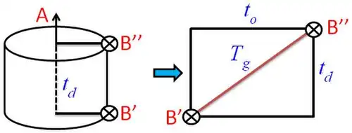
While B (satellite) has a circular orbit period t_o on a 2-axis plane (horizontal axis as 3-D space) around A (planet), it also follows a cylindrical orbit (from ${\displaystyle B'}$ to ${\displaystyle B''}$) around the A time-line (vertical) axis in hyper-sphere co-ordinates. A is moving with the universe expansion (along the time-line axis) at (v = c) but is stationary in 3-D space (v = 0). B is orbiting A at (v = c) but the time-line axis motion is equivalent (and so `invisible') to both A and B, and so for an observer the orbital period and orbital velocity measure is limited to 3-D space co-ordinates.

The age of the Planck universe and the observed universe differ by 5%.

${\displaystyle t_{Planck}}$ = 14.624 billion years

Age dilation:

${\displaystyle t_{\Lambda DCM}=t_{Planck}{\frac {v_{t}}{c}}}$ = 13.8 billion years

Hubble discrepancies (two different “frames”):

${\displaystyle H_{obs}=H_{4D}{\frac {v_{t}}{c}}}$

ΛCDM parameters from velocity-squared ratios:

${\displaystyle \sigma _{\Lambda }=({\frac {v_{t}}{c}})^{2}=(0.94365)^{2}}$ = 0.8905 (Tangential expansion energy)

${\displaystyle \sigma _{c}=({\frac {v_{r}}{c}})^{2}=(0.3309)^{2}}$ = 0.1095 (Radial gravitational energy)

${\displaystyle ({\frac {v_{t}}{c}})^{2}+({\frac {v_{r}}{c}})^{2}=1}$

References

- ↑ Macleod, Malcolm J.; "Programming cosmic microwave background parameters for Planck scale Simulation Hypothesis modeling". RG. Feb 2011. doi:10.13140/RG.2.2.31308.16004/7.
- ↑ Macleod, M.J. "Programming Planck units from a mathematical electron; a Simulation Hypothesis". Eur. Phys. J. Plus 113: 278. 22 March 2018. doi:10.1140/epjp/i2018-12094-x.
- ↑ Macleod, Malcolm J.; "Programming gravity for Planck unit Simulation Hypothesis modeling". RG. Feb 2011. doi:10.13140/RG.2.2.11496.93445/13.
- ↑ https://x.com/i/grok/share/jiSFBh30LBFRn2q13nTBY880I Grok AI analysis
- ↑ https://chatgpt.com/share/67e78967-0e78-8012-a665-c97421e0bef6 Chat AI analysis
- ↑ https://codingthecosmos.com/ai/deepseek-hypersphere.pdf Deepseek AI analysis
- ↑ https://codingthecosmos.com/ai/claude-hypersphere.pdf Claude AI analysis
- ↑ https://codingthecosmos.com/podcast/ Gemini generated podcast summaries