Understanding how to reduce tensor integrals to scalar integrals with the same number of external lines (renormalization)

Question

Currently in my QFT lecture, we are learning about the renormalization.

It was said that one-loop integrals in general can be reduced to scalar integrals, which are easier to solve. As an example I will consider the 2-point function.

The two-point function is:

$$B_0(p;m_0,m_1)=\frac{16\pi^2 \mu^{4-D}}{i}\int\frac{1}{(k^2-m_0)[(k + p)^2-m^2_1]}\frac{d^Dk}{(2\pi)^D}.$$

For the 2-point function we have the following relevant tensor integrals:

$$B_\mu(p;m_0,m_1)=\frac{16\pi^2\mu^{4-D}}{i}\int\frac{k_\mu}{(k^2-m_0)[(k + p)^2-m^2_1]}\frac{d^Dk}{(2\pi)^D}=B_1p_\mu$$

$$B_{\mu\nu}(p;m_0,m_1)=\frac{16\pi^2\mu^{4-D}}{i}\int\frac{k_\mu k_\nu}{(k^2-m_0)[(k + p)^2-m^2_1]}\frac{d^Dk}{(2\pi)^D}=B_{00}g_{\mu\nu}+B_11p_\mu p_\nu.$$

I have the 3 following questions:

1. If it is possible to illustrate $B_{\mu\nu}$ and $B_\mu$ (similarly as to how we can for $B_0$) via feynman diagrams, how would they look different?

2. When dealing with higher-order PT and the emergence of loops when we consider the higher-order feynman diagrams, in which scenarios would $B_\mu$ appear and in which $B_{\mu\nu}$? Or they appear both in a particular order?

3. Is there a physical interpretation difference between these tensor integrals, including the scalar one?

Answer 1

In this answer we sketch a recipe to remove the dependence of the loop momentum $k^{\mu}$ from a tensor numerator $N^{\mu_1\ldots\mu_r}(k)$ of a Lorentz covariant 1-loop Feynman diagram:

1. If the loop in the Feynman diagram contains $n$ propagators, use the Feynman parametrization to replace the $n$ denominator factors with just 1 denominator factor of the form $k^2+b\cdot k +c$.

2. Complete the square $k^2+b\cdot k +c=\left(k+\frac{b}{2}\right)^2+c-\frac{b^2}{4}$.

3. Shift the loop momentum integration variable $k^{\mu}+\frac{b^{\mu}}{2}\to k^{\mu}$ in the integral $\int_{\mathbb{R}^d}\!\frac{d^dk}{(2\pi)^d}$ so that the denominator becomes a function of the Lorentz invariant $k^2$.

4. We can now remove the antisymmetric part of the tensor numerator, i.e. we may assume that $N^{\mu_1\ldots\mu_r}(k)=N^{\mu_1\ldots\mu_r}(-k)$ is symmetric for $k^{\mu}\leftrightarrow -k^{\mu}$.

5. For rank $r=1$, the numerator $N^{\mu_1}$ is then a function of $k^2$, i.e. it is a scalar integral, cf. OP's question.

6. For rank $r=2$ and $r=3$, one can substitute $k^{\mu} k^{\nu} \to \frac{1}{d}g^{\mu\nu} k^2$ under the integral to reduce it to a scalar integral, cf. e.g. this Phys.SE post.

7. The above substitution trick can be generalized to higher tensor ranks $r$.

Answer 2

As you probably know, the $B$ integrals correspond to loop integrals with two propagators, which are usually called self-energy diagrams (though these loops do not appear only in self-energy calculations).

Thus, the denominator is always the same: $\frac{1}{[k^2 - m_0^2] [(k + p)^2 - m_1^2]} $. The only thing that can change is the numerator. Since we only have two propagators, and they must form a loop, the numerator will be given as the product of $N(k) = V_1(k) N_1(k) V_2(k) N_2(k) $ where $V_i(k)$ are the two vertex factors and $N_i(k)$ are the numerators of each propagator.

The case you wrote is $\lambda \phi^3$ theory, where the vertex is a constant factor and since you deal with scalar particles, the numerators are 1. Thus $N(k) = 1$ and you only get $B_0$ integrals.

Thus, the question is how to visualise the other integrals.

Let's start with $B_\mu$. In order to obtain this integral, we need $N(k) = k^\mu$. How can we achieve that? Well, the first example I can think of is to have a fermion propagator instead of a scalar one. So consider the self-energy of a fermion with a Yukawa interaction.

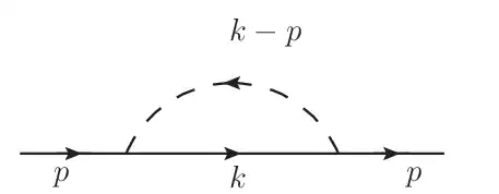
As before, the vertex and scalar propagator do not have $k$ dependence, but now the fermion propagator will give $N(k) = \gamma \cdot k + m$. So, ignoring constants, we will have the amplitude

$$\mathcal{M} = \gamma^\mu B_\mu + m B_0.$$

Here you can see that, in general, you will never find a single tensor integral but rather a combination of several ones. However, if you really want a Feynman diagram to illustrate $B_\mu$, you basically need to find a diagram for which $N(k)=k$.

A trivial example would be to just set $m=0$ in the previous example, but another option is the following diagram:

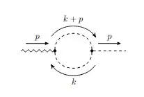
Similarly, you can find a lot of examples for $B_{\mu\nu}$. You just need to find diagrams with $N(k) = k^2$. Examples would be to have two fermion propagators (for example, the fermion loop contribution to the photon self-energy) or two sQED vertices (for example, the scalar loop contribution to the photon self-energy in sQED).

Regarding your second question. Keep in mind that the tensor integrals are single-loop integrals. Thus, you won't get anything from going to higher-order in PT.

Finally, I'm not sure what you mean in your last question, but something that could be interesting is that the degree of divergence is different for each of these integrals; for a B integral with $n$ indices, the degree of divergence will be $D-4+n$. So, a single parameter is able to renormalise the divergence from $B_0$ (as you know if you studied the renormalisation of $\lambda \phi^3$ for D=4). Two parameters are needed to renormalise $B_\mu$ (as you know if you studied the renormalisation of QED). And in general you will need three parameters to renormalise diagrams that involve $B_{\mu\nu}$. However, if you studied the renormalisation of QED, you know from the photon self-energy that symmetries are very important. Lorentz symmetry reduces the number of parameters from 3 to 2, and gauge invariance reduces further from 2 to 1, allowing you to renormalise QED.