When to average measurement results?

Question

What do I want to do?

I want to measure the gravitational acceleration $g$.
To do so I measure the fall time of an object from a height $h$, which I have measured previously up to a uncertainty $\sigma_h$.
I repeat this $n$ times and get $n$ different fall times $T_1, ... , T_n$. For sake of simplicity assume that these fall times have been measured exactly without a systematic measurement error, so that the only estimate for their uncertainty is their standard deviation.

What is my problem?

I can now come up with two different methods for combining my measurements to find a value for $g$. Obviously theory predicts $g=\frac{2h}{T^2}$.

Method 1

I first average my different time measurements $$\bar{T} = \frac{1}{n} \sum_i T_i,$$ calculate my best estimate for the uncertainty on the mean $$\sigma_{\bar{T}} = \sqrt{\frac{1}{n(n-1)}\sum_i (T_i-\bar{T})^2},$$ plug the nominal values for $\bar{T}$ and h into the above formula for $g$ to calculate my nominal value for $g$ and then do a gaussian error propagation to arrive at my result with uncertainty.

Method 2

I calculate $g_i$ for each of my measurements $T_i$. I then average the $g_i$. I find my statistical uncertainty in $\bar{g}$ by calculating $$\sigma_{\bar{g}}^{\text{stat}} = \sqrt{\frac{1}{n(n-1)}\sum_i (g_i-\bar{g})^2}.$$ I would then calculate my 'systematic' or correlated uncertainty caused by the uncertainty in $h$ by doing a Gaussian error propagation (or by parameter shifting?) but this time only in $h$.

Professors opinion/Conclusion

My professor told me that method 2 is invalid because the $g_i$ wouldn't be independent from each other (I assume method 2 then breaks down because i cant use the simple formula for the error on the mean of the $g_i$ if they are dependent, correct?). This dependence stems from the inclusion of $h$ in the formula for the $g_i$. But wouldn't this affect all measurements the same, essentially only shifting the $g_i$ by some factor, and wouldn't it thus still be correct to average them? If not, is there some other way to modify method 2, to make it correct? For example by using a different formula when computing the error on $\bar{g}$?
Also: Would both ways technically be unbiased estimators for g?
Related but sort of implies the opposite of what my professor said: When to average in the lab for indirect measurements?

Answer 1

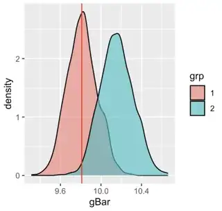
The problem of method 2 is not the uncertainty, but the bias: Due to the non-linear relationship $g \propto 1/t^2$ the error in the time measurement generates a non-symmetric distribution. Taking the average value of this non-symmetric distribution results in a systematic shift (=bias).

Personally, I find it most instructive to simulate the measurement. Here is a small R-code, which draws 2000 random samples and evaluates the two methods:

nSim = 2e3
height.target = 10     # [in m] height
height.sigma  =  0.05  # [in m] SD of height
height.true   = rnorm(nSim, mean=height.target, sd=height.sigma)
g.true = 9.81  # [in m/s^2]
h = 1/2gt^2
=> t = ...
time.true = sqrt(2*height.true/g.true)   # perfect time measurement
time.sigma = 0.15 # [in s] SD of time
time.meas  = rnorm(nSim, mean=time.true, sd=time.sigma)
time.mean  = mean(time.meas)
time.sd    = sd(time.meas)
h = 1/2gt^2
=> g = ...
Method 1:
g.mean  = 2*height.target/time.mean^2
gBar = g(h, tBar)
=> Var[gBar] = (dg/dh)^2 * Var[h] + (dg/dtBar)^2 * Var[tBar]
dgdh    = 2/time.mean^2
dgdt    = -22height.target/time.mean^3
gBar.sd = sqrt( dgdh^2height.sigma^2 + dgdt^2time.sigma^2/nSim )
cat(paste0("gBar = (", round.smartly(g.mean), '+/-', round.smartly(gBar.sd), 
           ') m/s^2\n'))
Method 2:
g.meas  = 2*height.target/time.meas^2
g.mean  = mean(g.meas)
g.sd    = sd(g.meas)
gBar.sd = g.sd/sqrt(nSim)
cat(paste0("gBar = (", round.smartly(g.mean), '+/-', round.smartly(gBar.sd), 
           ') m/s^2\n'))
Plot distribution:
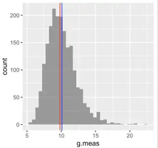
library(ggplot2)
DF = data.frame(g.meas)
gg = ggplot(DF, aes(x=g.meas)) + 
    geom_histogram(alpha=0.6, binwidth=histogram_binwidth(g.meas)) +
    geom_vline(xintercept=mean(g.meas), col="blue") +
    geom_vline(xintercept=9.81, col="red")
print(gg)

Method 1 yields $\bar g \pm \hat \sigma_{\bar g} \approx (9.78 \pm 0.067) m/s^2$ while method 2 yields $\bar g \pm \hat \sigma_{\bar g} \approx (10.1 \pm 0.052) m/s^2$. The bias is due to the uncertainty in the time measurement, which yields a non-symmetric distribution.

If we repeat the simulation 1000 times, but reduce the number of random samples per simulation to 200, we obtain the following graph, which clearly displays the bias.

Answer 2

I think that you are comparing estimating the error via a fractional uncertainty of (approximately) $\sqrt{\left(\dfrac{\sigma_{\rm h}}{h}\right)^2+2 \left(\dfrac{\sigma_{\rm T}}{T}\right)^2}$ for method $1$ and $\sqrt{\left(\dfrac{\sigma_{\rm h}}{h}\right)^2+ \left(\dfrac{\sigma_{\rm g}}{g}\right)^2}$ for method $2$.
You can see that there is a problem doing this in that you are not weighting the term $\left(\dfrac{\sigma_{\rm g}}{g}\right)^2$ enough given that the values of $g$ that you found were dependent on $T^2$ and you made measurements of $T$.
If you then decide to give a weighting of two to $\left(\dfrac{\sigma_{\rm g}}{g}\right)^2$ I think then that really does give weight to your Professor's objection to method $2$.
There is no uncertainty in period and height being uncorrelated.

Answer 3

The other answer is correct. The issue being identified there is that $g=g(h,T)$ so that then you cannot assume that $g$ and $h$ are independent variables suitable for the uncertainty combination that you want to apply. So the professor is correct.

But I want to comment that this is simply not the correct way to do the experiment you want to do.

Every time you reset the object back the $h$, you actually cannot know the $\delta h$ that you accidentally introduce. Of course, this is a tiny correction to $T$.

Instead, you should take a cluster of data for $h_1+\delta h$, so that you can find $\left<T_1\right>$ and the empirically determined $\sigma_{T_1}$ for it, and repeat for at least 5 quite different cases of $h$. In this way, and only in this way, can you argue that $\delta h$ is smaller than all the $h_2-h_1$ that you have considered, so that then you can ignore their contributions.

Then you plot $2h$ on the $x$-axis and $T^2$ with error bars $\sigma_{T^2}$ for them on the $y$-axis, and by linear regression with the constant term, extract $m=\frac1g$ from there. You have to show that the constant term is negligible; if it is not, then your experiment is broken. You cannot even flip $x$ and $y$ to get $g$ directly.

In fact, if the error bar plots $\sigma_{T^2}$ is not roughly constant magnitude, then you are very screwed. You might have to do a transformation to get what you want. In particular, it might be useful to explore $\sqrt{2h}$ v.s. $T$ just to see if the error bars will look more consistent in size. Then your gradient is $\frac1{\sqrt g}$, but at least the experiment will be well-done.

Note that the linear regression is done using the averaged, and thus smaller, dataset. You should not consider the clusters as separate data points on the plot, though it is useful and recommended to plot them so, just to visually see how the distribution looks like.