After analyzing the proposal of this question from various aspects, I fear that I have reached a negative answer for the use of the Lee-Yang theorem to study phase equilibria, particularly for the coexistence of three phases. I don't think this conclusion due to impossibility is definitive, but it is at least in the current state of knowledge.
In fact, as a specialist in thermodynamics, I have always welcomed any possibility of using statistical mechanics to evaluate macroscopic properties or make predictions about behavior. I have to recognize, however, that we greatly overestimate statistical models, which leave much to be desired in comparison with macroscopic empirical models for typically thermodynamic properties. I'm not talking about problems in the field of particle physics, but about the immense complexities of macroscopic models, such as predictions of melting or boiling temperatures.
In a nutshell, the critical temperature in Ising model is basically a temperature that makes the system pass from a magnetization order to the complete disorder. It is a completely different physical phenomenon from thermodynamical critical temperature, the threshold of the coexistence of vapor and liquid.
In the context of the Ising model, the concept of fugacity is not typically used in the same way as it is in the study of gases. The Ising model primarily deals with spins and their interactions, and the main focus is on quantities like magnetization, energy, and the partition function. However, we can discuss how zero fugacity, or a similar concept, would be interpreted within the framework of the Ising model. I write above about the generalization of Ising model suggested by Yvan Velenik.
The reason I say that it is not possible to apply the theory to the phase equilibria of water was the result that is observed when, instead of trying to enrich the statistical fugacity model, we use a real fugacity model, such as the equation by Van der Walls, which effectively changes phase. The Ising model, with the assumption of an ideal gas, definitely does not change phase, it is impossible to liquefy an ideal gas. I detail below what happens when you write the fugacities based on the Van der Waals equation and look for the zeros of that fugacity. In terms of macroscopic equations of state, it is even difficult to assign meaning to a "zero" of fugacity, a point at which pressure does not interfere with volume, unless very roughly emulating the lack of reaction of solids to pressure. The problem is that when this happens, the pressure itself and the phase diagram no longer make sense.
I don't think, however, that the answer I'm posting now is comfortable. I'm very unsatisfied with it and I even posted it as a rant. When we study "phases" in statistical mechanics, we expect them to be at least analogous to liquid and vapor phases in contact. The fact that they are so far away shows us how far we still have to go in science.
There is still one topic I would like to share about this analysis. Equations of state that involve phase change, such as Van der Waals or Peng Robinson, when looking for molar volumes for a given pressure and temperature, often offer complex solutions, but in totally different regions. For example, for water at one atmosphere, complex solutions start close to 500K, that is, close to the point we call the critical point (ver ábaco na imagem abaixo), when there is no longer a distinction between liquid and vapor. It is by no means a null fugitivity, but it is an appearance very similar to the results of the Lee-Yang analysis. Adaptation, however, would require a total reconstruction of the theory.
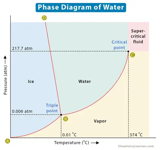
The idea of a critical temperature for the equations of state involves a point where the separation curve between liquid and vapor stops making sense, confusing the two phases. The fact that it is a point has always been somewhat embarrassing, because if we are at a point below the curve and go around this point in a circle, we go from vapor to liquid without realizing where the transition occurs. The idea of bringing an analysis analogous to Lee-Yang to molar volume transitions allows creating a dividing line between the regions of defined liquid and vapor, delimiting a region of undefined phase between vapor and liquid. At the end of this answer I show where the boundary defined by this line for the pressure of an atmosphere may be, according to some equations of state that clearly can equate the liquid and gaseous phases.
Let us deal with the details of the analysis.
Ising Model Overview
The Ising model is a mathematical model used in statistical mechanics to describe phase transitions in magnetic systems. It consists of discrete variables called spins, which can be in one of two states: +1 or -1. The spins are arranged on a lattice, and each spin interacts with its nearest neighbors.
The Hamiltonian (energy function) of the Ising model is given by:
$$ H = -J \sum_{\langle i,j \rangle} S_i S_j - h \sum_i S_i $$
where:
- $ J $ is the interaction strength between neighboring spins.
- $ h $ is the external magnetic field.
- $ S_i $ is the spin variable at site $ i $, which can be +1 or -1.
- The first sum is over all pairs of neighboring spins, and the second sum is over all spins in the lattice.
Partition Function in the Ising Model
The partition function $ Z $ for the Ising model is given by summing over all possible configurations of the spins, weighted by the Boltzmann factor $ e^{-\beta H} $, where $ \beta = \frac{1}{k_B T} $:
$$ Z = \sum_{\{S_i\}} e^{-\beta H} $$
Fugacity in the Ising Model
While fugacity is not directly used in the Ising model, we can draw an analogy by considering a parameter that adjusts the weight of configurations in a way similar to how fugacity affects the particle number in the grand canonical ensemble. In the Ising model, an analogous concept could be the external magnetic field $ h $.
Zero External Field
When the external magnetic field $ h $ is zero, the Hamiltonian simplifies to:
$$ H = -J \sum_{\langle i,j \rangle} S_i S_j $$
Physical Implications
- Symmetric States: With $ h = 0 $, the system has no preferred direction for the spins, leading to symmetry between the +1 and -1 spin states.
- Phase Transition: The Ising model exhibits a phase transition at a critical temperature $ T_c $. Below $ T_c $, the system spontaneously magnetizes, even without an external field. Above $ T_c $, the spins are disordered, and the net magnetization is zero.
- Partition Function Zeros: In the context of the Ising model, the zeros of the partition function $ Z $ can be analyzed in the complex plane (often using techniques like Lee-Yang zeros). These zeros provide insight into the phase transition behavior.
Zero Fugacity Analogy
If we draw an analogy with fugacity in the grand canonical ensemble, zero fugacity would correspond to a situation where the contribution of certain configurations is entirely suppressed. In the Ising model with $ h = 0 $:
- Symmetric Contributions: Both spin-up and spin-down configurations contribute equally to the partition function.
- Critical Phenomena: The phase transition occurs due to the collective behavior of spins rather than the influence of an external field.
In the Ising model, the concept of fugacity is not directly applicable. However, we can draw an analogy with the external magnetic field $ h $. When $ h = 0 $, the system exhibits symmetric behavior between spin states and undergoes a phase transition driven by temperature. The zeros of the partition function in the complex plane provide insights into the phase transition, similar to how fugacity zeros are used to understand phase transitions in other contexts. The Ising model focuses on the interplay between thermal fluctuations and spin interactions to describe critical phenomena and phase transitions.
Yvan Velenik gave me some hope with the paper on generalizations of the Ising model. The generalization is, however, the Blume-Capel model, still very far from the macroscopic phase change. Additionally to the possibility of magnetization or complete disorganization, there is a third state.
The Blume-Capel model is an extension of the Ising model in statistical mechanics. It includes an additional term that allows for the spins to take on a value of 0, in addition to the usual ±1 values. This model is used to study phase transitions and critical phenomena in systems where spin states can vary in this more complex manner.
Key Features of the Blume-Capel Model
- Spin States: Unlike the Ising model, which has spins $ S_i $ that can be either +1 or -1, the Blume-Capel model allows the spins to take on three possible values: +1, 0, or -1.
- Hamiltonian: The Hamiltonian (energy function) for the Blume-Capel model is given by:
$$ H = -J \sum_{\langle i,j \rangle} S_i S_j + D \sum_i S_i^2 - h \sum_i S_i $$
- $ J $ is the interaction strength between neighboring spins.
- $ \langle i,j \rangle $ indicates summation over nearest neighbor pairs.
- $ D $ is the single-ion anisotropy parameter, which controls the energy cost of the $ S_i = 0 $ state.
- $ h $ is an external magnetic field.
- $ S_i $ can take values in {+1, 0, -1}.
Physical Interpretation
- Interaction Term: The first term, $-J \sum_{\langle i,j \rangle} S_i S_j$, is similar to the Ising model and represents the interaction between neighboring spins.
- Single-Ion Anisotropy Term: The second term, $ D \sum_i S_i^2 $, represents the energy associated with the spin taking the value 0. When $ D $ is large and positive, the system prefers to have more spins in the 0 state.
- External Field Term: The third term, $-h \sum_i S_i$, represents the effect of an external magnetic field.
Phase Transitions
The Blume-Capel model exhibits rich phase behavior, with different phases depending on the temperature $ T $, the anisotropy parameter $ D $, and the interaction strength $ J $. Key phases include:
- Ferromagnetic Phase: At low temperatures and low values of $ D $, the spins tend to align, resulting in a non-zero net magnetization.
- Paramagnetic Phase: At high temperatures, thermal fluctuations dominate, leading to a disordered phase with zero net magnetization.
- Intermediate Phases: Depending on the values of $ D $ and $ T $, the model can exhibit intermediate phases where spins take the value 0, leading to mixed phases.
The fugacity of a substance provides a measure of its tendency to escape or expand and is often used to correct the ideal gas law to account for real gas behavior. For a Van der Waals gas, the fugacity can be calculated using the Van der Waals equation of state. Here is the step-by-step process for calculating the fugacity of water modeled by the Van der Waals equation:
Van der Waals Equation
The Van der Waals equation of state is:
$$ \left( P + \frac{a}{V_m^2} \right) (V_m - b) = RT $$
where:
- $ P $ is the pressure,
- $ V_m $ is the molar volume,
- $ T $ is the temperature,
- $ R $ is the universal gas constant,
- $ a $ and $ b $ are the Van der Waals constants specific to the substance.
Fugacity Calculation
Expressing Fugacity:
Fugacity $ f $ is related to the pressure $ P $ and can be expressed as:
$$ \ln \frac{f}{P} = \frac{1}{RT} \int_{V_m}^{\infty} \left( Z - 1 \right) \frac{dV_m}{V_m} $$
where $ Z $ is the compressibility factor:
$$ Z = \frac{PV_m}{RT} $$
Compressibility Factor $ Z $:
For a Van der Waals gas:
$$ Z = \frac{PV_m}{RT} = \frac{P(V_m - b)}{RT} $$
Fugacity Coefficient $ \phi $:
The fugacity coefficient $ \phi $ is defined as:
$$ \phi = \frac{f}{P} $$
Thus:
$$ \ln \phi = \frac{1}{RT} \int_{V_m}^{\infty} \left( Z - 1 \right) \frac{dV_m}{V_m} $$
Integral Calculation:
To calculate the integral, we need to express $ Z - 1 $ and integrate with respect to $ V_m $.
Detailed Steps
Van der Waals Equation:
Solve the Van der Waals equation for $ V_m $ given $ P $ and $ T $.
Compressibility Factor:
$$ Z = \frac{P(V_m - b)}{RT} $$
Fugacity Coefficient:
The integral becomes:
$$ \ln \phi = \frac{1}{RT} \int_{V_m}^{\infty} \left( \frac{P(V_m - b)}{RT} - 1 \right) \frac{dV_m}{V_m} $$
Substitute $ Z $ and simplify:
$$ \ln \phi = \frac{P}{RT} \int_{V_m}^{\infty} \left( \frac{V_m - b}{V_m} - \frac{RT}{P} \frac{1}{V_m} \right) dV_m $$
Separate the integral:
$$ \ln \phi = \frac{P}{RT} \left( \int_{V_m}^{\infty} \frac{V_m - b}{V_m} dV_m - \int_{V_m}^{\infty} \frac{RT}{P} \frac{1}{V_m} dV_m \right) $$
Evaluating the Integral:
Evaluate each part of the integral separately.
For the first part:
$$ \int_{V_m}^{\infty} \frac{V_m - b}{V_m} dV_m = \int_{V_m}^{\infty} \left( 1 - \frac{b}{V_m} \right) dV_m $$
This simplifies to:
$$ \int_{V_m}^{\infty} dV_m - b \int_{V_m}^{\infty} \frac{dV_m}{V_m} $$
The first integral diverges, so we use limits or an appropriate cutoff.
For the second part:
$$ -\int_{V_m}^{\infty} \frac{RT}{P} \frac{1}{V_m} dV_m = -\frac{RT}{P} \ln V_m $$
Combining Results:
Combine the results to get:
$$ \ln \phi = \frac{P}{RT} \left( V_m - b \ln V_m \right) - \ln V_m $$
Fugacity:
Finally, the fugacity is:
$$ f = \phi P $$
Exploring the zeros of the fugacity analytically in the Van der Waals model involves delving into the conditions under which the fugacity coefficient, $ \phi $, becomes zero. This exploration is important because it helps understand phase transitions and critical phenomena in real gases.
The Van der Waals equation of state is:
$$ \left( P + \frac{a}{V_m^2} \right) (V_m - b) = RT $$
For fugacity $ f $ and fugacity coefficient $ \phi $, the relationships are:
$$ f = \phi P $$
$$ \ln \phi = \frac{1}{RT} \int_{V_m}^{\infty} \left( Z - 1 \right) \frac{dV_m}{V_m} $$
To explore the zeros of the fugacity coefficient, we need to understand the conditions under which the integral expression for $ \ln \phi $ can lead to $ \phi $ being zero. However, analytically solving this directly is highly non-trivial. We can, instead, look for insights by analyzing the behavior of the compressibility factor $ Z $ and the nature of the Van der Waals equation.
Step-by-Step Analytical Exploration
Compressibility Factor $ Z $:
The compressibility factor $ Z $ is given by:
$$ Z = \frac{PV_m}{RT} $$
Rewriting the Van der Waals Equation:
We can express the Van der Waals equation in terms of $ Z $:
$$ Z = \frac{P(V_m - b)}{RT} $$
Substituting this into the Van der Waals equation, we get:
$$ Z = 1 + \frac{a}{RTV_m} \left( \frac{1}{V_m} \right) $$
Integral for $ \ln \phi $:
The expression for $ \ln \phi $ involves integrating the deviation of $ Z $ from unity:
$$ \ln \phi = \frac{1}{RT} \int_{V_m}^{\infty} \left( Z - 1 \right) \frac{dV_m}{V_m} $$
Finding Zeros:
For $ \phi $ to be zero, $ \ln \phi $ must be negative infinity, which means the integrand must lead to an infinite negative contribution. This would imply conditions where $ Z $ diverges or where the integral behaves pathologically.
Simplifying Assumptions and Analysis
Critical Points and Phase Transitions:
Near the critical point, the behavior of the Van der Waals equation changes significantly. The critical point is where:
$$ \left( \frac{\partial P}{\partial V_m} \right)_{T_c} = 0 $$
$$ \left( \frac{\partial^2 P}{\partial V_m^2} \right)_{T_c} = 0 $$
Behavior Near Critical Point:
At the critical point, the compressibility factor $ Z $ approaches a critical value $ Z_c $, and the system exhibits critical phenomena. For the Van der Waals gas, the critical compressibility factor is typically:
$$ Z_c = \frac{3}{8} $$
Complex Fugacity:
Introducing a complex fugacity $ z = e^{\beta \mu} $ allows for the analysis of Lee-Yang zeros. The partition function can be analyzed for zeros in the complex fugacity plane. Maybe there was a way to do this. If you have any clue, please tell me.
The interesting possibility of a Lee-Yang's type analysis for the volumes in EOS that are able to simulate liquids.
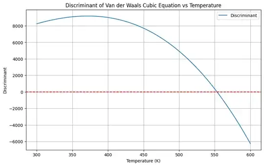
To determine the temperature range at 1 atm for which the Van der Waals equation yields complex solutions for the molar volume $ V_m $, we need to analyze the roots of the cubic equation derived from the Van der Waals equation. Complex solutions typically arise when the discriminant of the cubic equation is negative.
Van der Waals Equation
The Van der Waals equation for real gases is given by:
$$ \left( P + \frac{a}{V_m^2} \right) (V_m - b) = RT $$
Rewriting it in the form of a cubic polynomial:
$$ P V_m^3 - (P b + R T) V_m^2 + a V_m - a b = 0 $$
Discriminant of a Cubic Equation
For a cubic equation of the form $ Ax^3 + Bx^2 + Cx + D = 0 $, the discriminant $\Delta$ determines the nature of its roots:
- If $\Delta > 0$, the equation has three distinct real roots.
- If $\Delta = 0$, the equation has a multiple root, and all its roots are real.
- If $\Delta < 0$, the equation has one real root and two non-real complex conjugate roots.
The discriminant $\Delta$ for a cubic equation $Ax^3 + Bx^2 + Cx + D = 0$ is given by:
$$ \Delta = 18ABCD - 4B^3D + B^2C^2 - 4AC^3 - 27A^2D^2 $$
Applying to Van der Waals Equation
Let's compute the discriminant for the Van der Waals cubic equation and determine the temperatures at which it becomes negative (indicative of complex solutions).
- Define Constants and Temperature Range: We will consider a broad temperature range.
- Calculate the Discriminant: Compute the discriminant for each temperature.
- Determine Temperature Range: Identify the temperatures where the discriminant is negative.
Here is the Python code to perform these steps:
import numpy as np
import matplotlib.pyplot as plt
Constants
a = 5.536  # L^2 atm / mol^2
b = 0.03049  # L / mol
R = 0.0821  # L atm / K mol
P = 1  # atm
Temperature range (in Kelvin)
T_range = np.linspace(300, 600, 300)  # Adjust the range as needed
Function to calculate the discriminant of the Van der Waals cubic equation
def discriminant(P, b, R, T, a):
    A = P
    B = -(P * b + R * T)
    C = a
    D = -a * b
    return (18 * A * B * C * D) - (4 * B3 * D) + (B2 * C2) - (4 * A * C3) - (27 * A2 * D2)
Calculate discriminant for each temperature
discriminants = [discriminant(P, b, R, T, a) for T in T_range]
Determine the temperature range where the discriminant is negative
complex_solution_temperatures = T_range[np.array(discriminants) < 0]
Plotting discriminant
plt.figure(figsize=(10, 6))
plt.plot(T_range, discriminants, label='Discriminant')
plt.axhline(0, color='red', linestyle='--')
plt.xlabel('Temperature (K)')
plt.ylabel('Discriminant')
plt.title('Discriminant of Van der Waals Cubic Equation vs Temperature')
plt.legend()
plt.grid(True)
plt.show()
Display the temperature range with complex solutions
print("Temperature range with complex solutions (in Kelvin):")
print(complex_solution_temperatures)
Expected Outcome
- The plot will show the discriminant as a function of temperature.
- The horizontal red dashed line at zero helps identify when the discriminant crosses from positive to negative values.
- The temperatures where the discriminant is negative indicate the range where the Van der Waals equation has complex solutions.
By running this code, you will obtain the temperature range where the Van der Waals equation predicts complex solutions for the molar volume at 1 atm pressure. This analysis helps understand the phase behavior of water and other substances under different conditions and may plot a delimitation of a region on the phase diagram of well defined liquids and gases and a "no men's land".
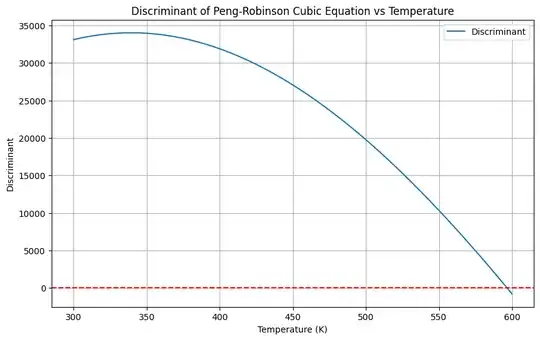
Peng Robinson prediction of de dividing line for well defined phases
It is possible, too, to perform the same evaluation for the Peng-Robinson equation. The Peng-Robinson equation of state is another cubic equation of state used to describe the behavior of real gases. The Peng-Robinson equation is given by:
$$ P = \frac{RT}{V_m - b} - \frac{a(T)}{V_m (V_m + b) + b(V_m - b)} $$
where:
- $ P $ is the pressure,
- $ V_m $ is the molar volume,
- $ R $ is the universal gas constant,
- $ T $ is the temperature,
- $ a(T) $ and $ b $ are substance-specific constants.
The temperature dependence of $ a $ is given by:
$$ a(T) = a_c \left[ 1 + \kappa \left( 1 - \sqrt{\frac{T}{T_c}} \right) \right]^2 $$
where:
- $ a_c $ is the value of $ a $ at the critical temperature,
- $ T_c $ is the critical temperature,
- $ \kappa $ is an empirically derived factor.
The constants $ a_c $, $ b $, and $ \kappa $ for water can be determined from its critical properties:
- $ T_c $ = 647.096 K,
- $ P_c $ = 22.064 MPa,
- $ R $ = 0.0821 L atm / K mol,
- $ a_c $ and $ b $ are derived from critical conditions.
For water, the constants are approximately:
- $ a_c $ = 0.45724 $\frac{R^2 T_c^2}{P_c}$,
- $ b $ = 0.07780 $\frac{R T_c}{P_c}$,
- $ \kappa $ is empirically derived from the acentric factor.
To find the roots of the Peng-Robinson equation and determine when complex roots occur, we follow a similar approach:
- Define Constants and Temperature Range.
- Calculate the Discriminant of the cubic equation derived from the Peng-Robinson equation.
- Identify Temperature Range where the discriminant is negative.
Here is the Python code to perform these steps:
import numpy as np
import matplotlib.pyplot as plt
Constants
R = 0.0821  # L atm / K mol
P = 1  # atm
T_c = 647.096  # K
P_c = 22.064 * 10  # atm
omega = 0.344  # acentric factor for water
Calculate a_c and b
a_c = 0.45724 * (R2 * T_c2) / P_c
b = 0.07780 * (R * T_c) / P_c
Calculate kappa
kappa = 0.37464 + 1.54226 * omega - 0.26992 * omega**2
Temperature range (in Kelvin)
T_range = np.linspace(300, 600, 300)  # Adjust the range as needed
Function to calculate a(T)
def a(T):
    return a_c * (1 + kappa * (1 - np.sqrt(T / T_c)))**2
Function to calculate the discriminant of the Peng-Robinson cubic equation
def discriminant_peng_robinson(P, b, R, T, a_T):
    A = P
    B = -(R * T - P * b)
    C = a_T - 3 * b2 * P - 2 * b * R * T
    D = -a_T * b + b2 * R * T + b3 * P
    return (18 * A * B * C * D) - (4 * B3 * D) + (B2 * C2) - (4 * A * C3) - (27 * A2 * D**2)
Calculate discriminant for each temperature
discriminants = [discriminant_peng_robinson(P, b, R, T, a(T)) for T in T_range]
Determine the temperature range where the discriminant is negative
complex_solution_temperatures = T_range[np.array(discriminants) < 0]
Plotting discriminant
plt.figure(figsize=(10, 6))
plt.plot(T_range, discriminants, label='Discriminant')
plt.axhline(0, color='red', linestyle='--')
plt.xlabel('Temperature (K)')
plt.ylabel('Discriminant')
plt.title('Discriminant of Peng-Robinson Cubic Equation vs Temperature')
plt.legend()
plt.grid(True)
plt.show()
Display the temperature range with complex solutions
print("Temperature range with complex solutions (in Kelvin):")
print(complex_solution_temperatures)
Expected Outcome
- The plot will show the discriminant as a function of temperature.
- The horizontal red dashed line at zero helps identify when the discriminant crosses from positive to negative values.
- The temperatures where the discriminant is negative indicate the range where the Peng-Robinson equation has complex solutions.