I've asked a question before which was ''The proof of KVL,'' and the answer was if that we are dealing with electrostatic field then it's conservative field, and the closed line integral is equal to zero $$ \oint\vec{E} \cdot d\vec{l}=0.$$ But what happens if we are dealing with a changing magnetic field? According to Faraday's Law, $$\oint\vec{E} \cdot d\vec{l}=-\frac{d\Phi_{B}}{dt}.$$ in this case we are not dealing with an conservative field, so the sum of line integrals in any loop will not equal to zero and consequently the sum of voltages across the loop will not equal to zero which can be written mathematically as $$\oint_{C}\vec{E} \cdot d\vec{l}=\sum_{i}^{N}\int_{C_{i}}^{}\vec{E}\cdot d\vec{l}=\sum_{i}^{N}V_{i}=-\frac{d\Phi_{B} }{dt}.$$ So then is the KVL applicable in this cases?
3 Answers
If the region of the domain where the magnetic field is not negligible is limited in space you can usually isolate these regions from the regions if space where the electric field is irrotational, and you can user voltage and current Kirchhoff laws.
As an example, assume that you have a part of a circuit where the magnetic field $\mathbf{b}(\mathbf{r})$ is non-zero, and the motion of a part of the circuit makes the flux vary, producing a electromotive force, following Faraday's law.
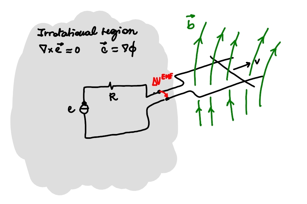
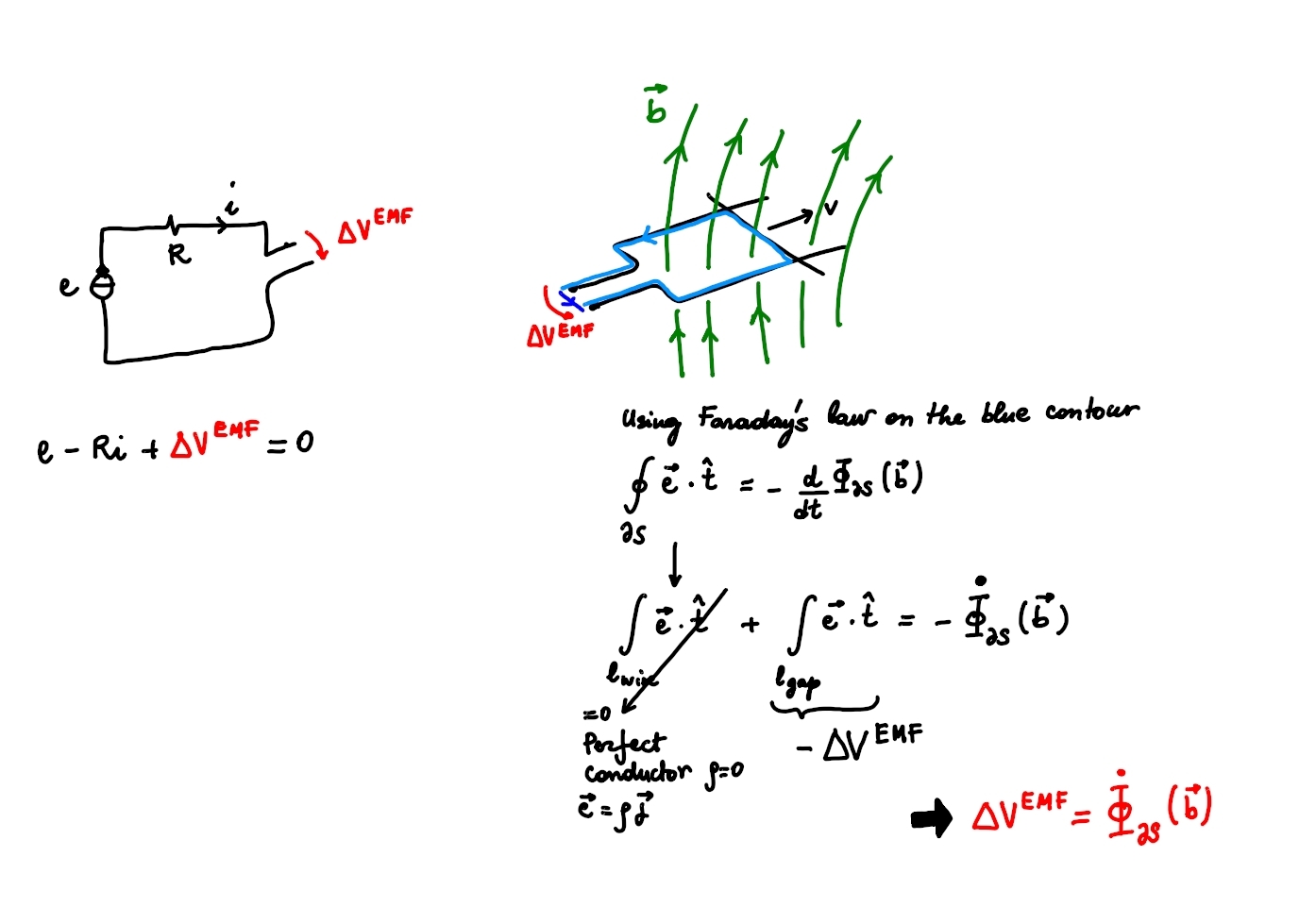
Let's first analyze the rotational region of the domain using Faraday's law, applied to the close geometrical contour built with the conductor wire $\ell_{wire}$ and the segment $\ell_{gap}$ joining the two extreme point of the conductor, $\delta S = \ell_{wire} \cup \ell_{gap}$
$\displaystyle -\dot\Phi_{S}(\mathbf{b}) = -\dfrac{d}{dt} \int_S \mathbf{b} \cdot \mathbf{\hat{n}} = \oint_{\partial S} \mathbf{e}^* \cdot \mathbf{\hat{t}} = \underbrace{\int_{\ell_{wire}} \mathbf{e}^* \cdot \mathbf{\hat{t}}}_{= 0, \text{ for perfect conductors}} + \int_{\ell_{gap}} \mathbf{e} \cdot \mathbf{\hat{t}} = - \Delta V^{EMF}$.
Now that we have found the expression of the potential difference across the two ends of the conductors, we can study the part of the circuit in the irrotational regions with Kirchhoff laws. Here, using KVL, we find
$0 = e - Ri + \Delta V^{EMF} = e - Ri + \dot \Phi_{\partial S} (\mathbf{b})$.
EDIT: the right formulation of the integral form of Faraday's law, coming from the differential equation
$\nabla \times \mathbf{e} = -\dfrac{\partial \mathbf{b}}{\partial t}$
reads
$\displaystyle - \dfrac{d}{dt} \underbrace{\int_S \mathbf{b} \cdot \mathbf{\hat{n}}}_{\Phi_{S} (\mathbf{b})} = \underbrace{\oint_{\partial S} \left( \underbrace{\mathbf{e} + \mathbf{v}_s \times \mathbf{b}}_{\mathbf{e}^*} \right) \cdot \mathbf{\hat{t}}}_{EMF_{\partial S}}$$\quad \rightarrow \quad $$\dot{\Phi}_{S} (\mathbf{b}) = - EMF_{\partial S}$.
This expression comes from the right application of the formulas for time derivation of integrals over domains that are moving in space, here for time derivative of a flux of a vector field $\mathbf{b}$ on a moving surface $S$ that reads
$\displaystyle \frac{d}{dt} \int_{S(t)} \mathbf{b} \cdot \mathbf{\hat{n}} = \int_{S(t)} \dfrac{\partial \mathbf{b}}{\partial t} \cdot \mathbf{\hat{n}} + \int_{S(t)}(\nabla \cdot \mathbf{b}) \ \ \mathbf{v}_s \cdot \mathbf{\hat{n}} - \oint_{\partial S(t)} \mathbf{v}_S \times \mathbf{b}$
For the proof of the expression above, you can take a look here: https://basics.altervista.org/test/Math/time_derivatives_of_integrals/time_derivatives_of_integrals.html.
For the magnetic field, the second term on the right-hand side is identically equal to zero, since $\nabla \cdot \mathbf{b} = 0$.
- 13,368
KVL is a circuital law. You need to define a circuit path, let's call it $\Gamma$, that joins your circuital components. If you can find a path $\Gamma$ that does not link the changing magnetic flux, then you can use KVL on that path and the sum of all voltages across your components' terminals will end up being zero.
Note: apart from a minor sign change, in the following I am using the definition of voltage given by the International Electrotechnical Commission (IEC) and by the International Standard Organization (ISO, standards ISO 8000-1 and ISO 8000-6):
https://www.electropedia.org/iev/iev.nsf/display?openform&ievref=121-11-27
(Incidentally it is also the definition of voltage that can be found on the German Wikipedia page).
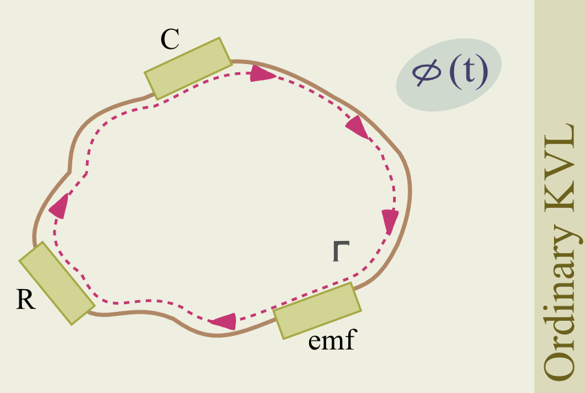
Ordinary KVL
When there is no magnetic flux present in your circuit and components we can express 'ordinary KVL' as: $$ \oint_{\Gamma}\vec{E}.\vec{dl}=0 $$ In fact, we can decompose this closed path into the partial paths going through each component; after accounting for all the signs, we will end up with EMF when we go through a battery, an ohmic voltage drop when we go through a resistor and a capacitor voltage when we go through a capacitor... $$ \int_{battery}\vec{E}.\vec{dl} + \int_{resistor}\vec{E}.\vec{dl} + \int_{capacitor}\vec{E}.\vec{dl} =0 $$
 C
C
...and their sum (with appropriate signs) will be zero, as stated by 'ordinary KVL'.
As a side note, in this conservative setting, all integrals relative to resistors and capacitors are path-independent and we can either integrate along the path going through the components or jumping across the terminals.
Extended KVL
Whenever a changing magnetic flux is present and is linked by the circuit path $\Gamma$, 'ordinary KVL' no longer applies because the circulation of E is no longer zero, as stated by Faraday's law: $$ \oint_{\Gamma=\partial\Sigma}\vec{E}.\vec{dl}=-\frac{d}{dt}\iint_\Sigma \vec{B}.\vec{dS}=-\frac{d\phi}{dt} $$
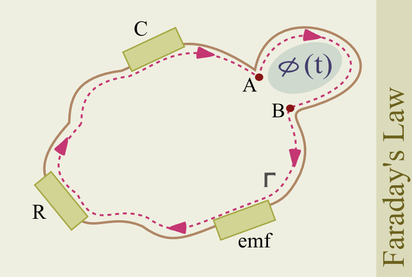
In most (but not all) cases, though, it is possible to define a new circuit path $\Gamma'$ in such a way that no appreciable (changing) magnetic flux is linked by it; in order to do that we will have to introduce one or more new components - that I will call 'magnetic components' for short - that will conceal the magnetic flux inside them. We end up with a new circuit that will link all non-magnetic components as before (by either going through them or jumping at their terminals, as you prefer) but will definitely skip the interior of the magnetic ones by 'jumping' at their terminals.
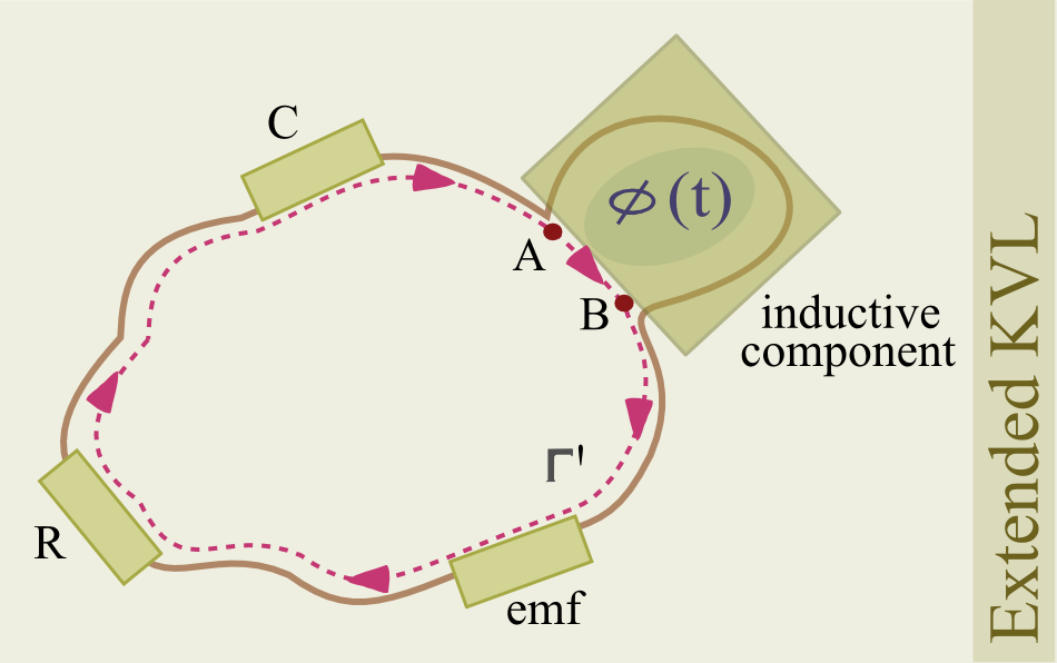
Since the new circuit path $\Gamma'$ joins all components without linking any of the changing flux we can write: $$ \int_{\Gamma'}\vec{E}.\vec{dl}=0 $$ This is an expression of 'extended KVL' and, as before, we can break up the integral into partial segments that represent the various components, but will always 'skip' the magnetic components by jumping at their terminals in order to leave the magnetic flux region out of the circuit's path. $$ \int_{battery}\vec{E}.\vec{dl} + \int_{resistor}\vec{E}.\vec{dl} + \int_{capacitor}\vec{E}.\vec{dl}+ \int_{jump_{A->B}}\vec{E}.\vec{dl} =0 $$ Now, here comes the neat trick: we express the path integral along the 'jump' at the magnetic component's terminals in terms of the inner - and hidden from the circuit's path $\Gamma'$ - changing magnetic flux. I am going to do it in the simplest of magnetic component: a coil linking an externally generated variable magnetic flux (not a self-inductor, and neither the secondary of a transformer, but a magnetic sensor).
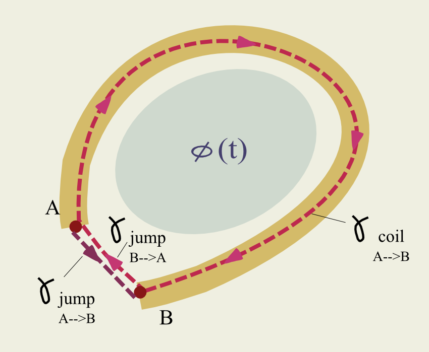
How do we compute the path integral of E.dl along the jump at its terminals? Simple: we compute the circulation of E.dl along the closed path formed by said jump and the coil's conductor invoking Faraday's law $$ \int_{coil_{A->B}}\vec{E}.\vec{dl}+\int_{jump_{B->A}}\vec{E}.\vec{dl}=\oint_{\partial\Sigma}\vec{E}.\vec{dl}=-\frac{d\phi}{dt} $$ and then we subtract the path integral of E.dl along the coil's conductor: if the conductor is perfect, the electric field inside of it will be zero and the path integral will be... zero. By reversing the endpoints of the path (because we want $\Gamma'$ to proceed from A to B, like $\Gamma$ did, we end up with $$ \int_{jump_{A->B}}\vec{E}.\vec{dl}=-\int_{jump_{B->A}}\vec{E}.\vec{dl}=+\frac{d\phi}{dt} $$ And we can pretend this is a voltage drop just like the ones for resistors and capacitors.
Let's compare the two ways to treat a circuit with lumped magnetic components: The purist will apply Faraday's law directly
Figure 5+3 = 8
The practitioner will fold back to the 'extended KVL' for the amended path $\Gamma'$ in the following form
Figure 5+3-8=0
No KVL
Now let's go back to the derivation of the voltage across our coil. Observe carefully: if you accept the definition of voltage as the path integral of the total electric field along a given path (see my answer here for the definition of voltage in line with the IEC definitions) you have one value of voltage across the coil's terminals (let's call it $V_L$), and a different value of voltage along the coil itself (zero, in a perfect conductor). This difference makes sense because the electric field is no longer conservative and so its line integrals are in general path-dependent.
Since we end up with two different values of voltage for paths with the same endpoints, it is clear that, inside a magnetic component, KVL is no longer applicable. And yet, thanks to our trick of skipping the innards of such components, 'extended KVL' still works when applied to the modified circuit path $\Gamma'$ . (This is why Feynman, in chapter 22 of the second volume of his lectures, insists that in order to use circuital simplifications no magnetic fields must escape the lumped components.)
Are there circuits that are not 'KVL-amendable'? The answer is yes: one example of such a circuit is a ring with two opposing resistors (or capacitors, or inductors, or a mix of the above) connected by a circuit path $\Gamma$ that is required to link a variable magnetic flux region.
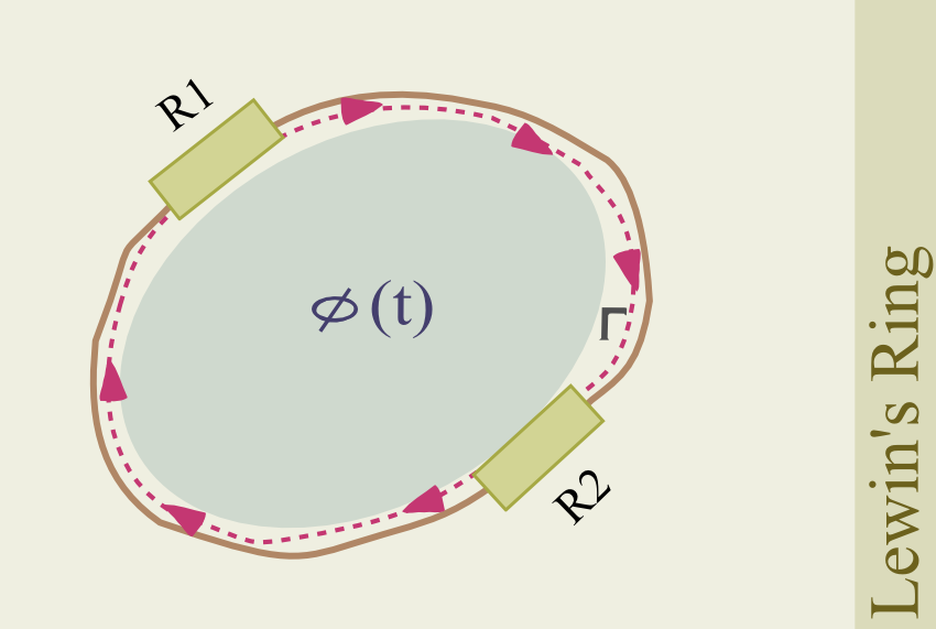
This constraint, which can be enforced in practice by requiring that the two resistors be on the opposite sides of a conductive ring that is strictly embracing the tube of flux that is delimiting the magnetic flux region makes it impossible to define a circuit path $\Gamma'$ that excludes the magnetic flux region without changing the nature of the circuit.
This is the circuit used by Walter Lewin in his much discussed superdemo, and it is an example of unlumpable circuit for which KVL does not apply. The voltage associated with a path that goes through the left resistor will be different from the voltage associated with a path (with the same endpoints!) that goes through the right resistor.
If you are able to define a circuit path that goes through the resistors but does not encircle the variable magnetic region, like in the following picture
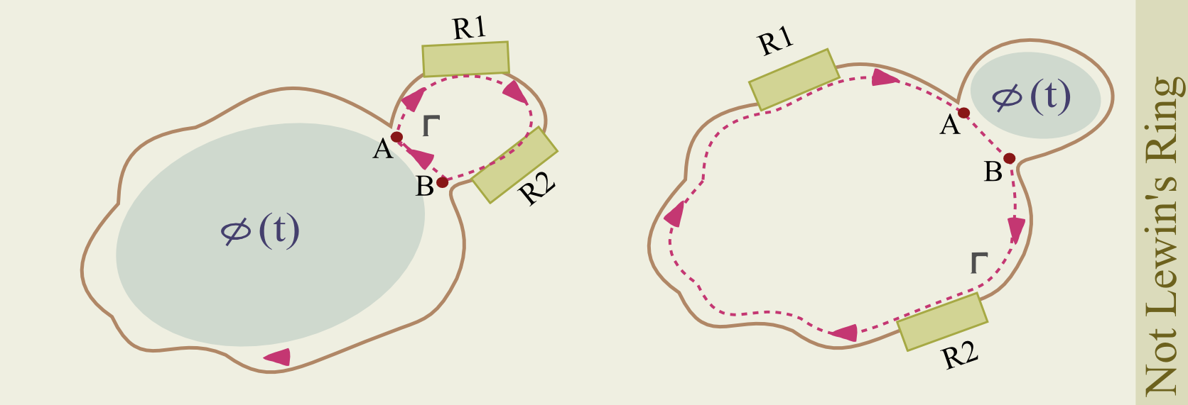
then you are not considering Lewin's ring. The above two circuits can be modeled with ordinary lumped parameter circuits, where the portion of conductor that goes around the magnetic region is modeled by a coil or the secondary of a transformer. This is not possible in the case of Lewins' ring.
Let me stress this: the V in KVL stands for voltage and, according to the IEC definition, voltage is the path integral of the total electric field (and not its conservative component $\vec{E}_c=\vec{E}-(-\partial\vec{A}/\partial{t})$ alone, which is responsible for the scalar potential difference.) If you compare the path integrals of the conservative component $E_c$ you will find that they are path independent, and will give the same result of the scalar potential difference between the same two points on the ring.
Measuring addendum
The IEC/ISO definition of voltage gives consistent results in accordance with what is read by a voltmeter, regardless of the source of the 'electromotance'.
Consider for example the following two circuits, one where the source of EMF is the lumped secondary coil of a transformer, and one where the circuit path encloses the variable magnetic region:
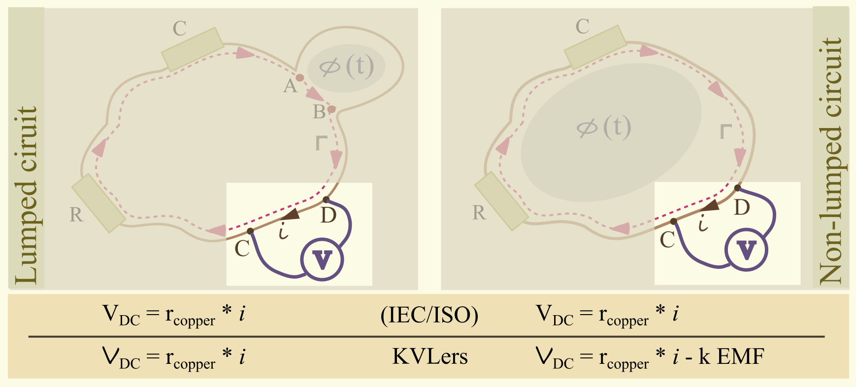
If you only have access to, say, one eight of the length of the copper conductor forming joining the components in a room without knowledge of what is outside, can you find the voltage between points C and D, assuming the current in the circuit is not generating a relevant dB/dt of its own (say it's 10mA at 50Hz)?
Using the IEC/ISO definition of voltage you get consistent results in both cases: the IEC voltage is in both cases equal to what Ohm's law tell you, and it is also equal to what you measure with a voltmeter in your room.
Using the 1800s version of voltage that is equal to scalar potential difference in the IEC notations, you cannot tell what it is unless you know whether the EMF is localized or distributed. And you can't trust your voltmeter either because it does not measure 'your'version of voltage.
References:
Ramo, Whinnery, VanDuzer, "Fields and Waves in Communication Electronics", Wiley. p. 266 in the first edition, Chapter 4 "The electromagnetics of circuits" in the second and third editions.
Purcell, Morin, "Electricity and Magnetism", Cambridge
Feynman, "Feynman's Lectures on Physics", Addison Wesley. Volume 2 , Chapter 22.
Popovic, "Introductory Engineering Electromagnetics", Addison Wesley, p. 496
Brandão Faria, "Electromagnetic Foundations of Electrical Engineering", Wiley, p. 208
- 906
This is a frequent question and often people are quite confused about it. The way to clear up confusion and answer the question starts with realizing what voltage in the KVL means.
The voltages referred to in KVL are meant to be unique numbers for each pair of points in space; they are actually differences of electric potential $\varphi$. Potential is a single-valued function of position, so summing up all changes of potential in a closed path, we have to get zero. So KVL is really a trivial consequence of what we mean by voltage when working with circuits.
There is another concept of voltage (IEC voltage), based on net electric field, which is a path-dependent concept; when you have different paths connecting point 1 to point 2, these different paths have different voltages. This is not what V means in KVL; voltage in KVL has unique value for each pairs of points in the circuit, it does not depend on the path joining them.
Voltage for pair of points in a circuit 1,2 can be calculated from electric fields in two different ways:
- we use the IEC voltage restricted to a special path: we integrate net electric field over a special path $p_{special}$ going from 1 to 2, for which the induced electric field contribution is zero, so KVL voltage for the ordered pair of points (1,2) is
$$ V = \int_{p_{special}} \mathbf E \cdot d\mathbf s. $$
- we integrate the conservative component of electric field $\mathbf E_c$ over any path starting at 1 and ending in 2, which shows manifestly that voltage in KVL is a drop of electric potential $\varphi$ when going from 1 to 2:
$$ V = \int_{p}\mathbf E_c \cdot d\mathbf s = \varphi_1 - \varphi_2. $$
Both ways give the same value of voltage (the special path $p_{special}$ is such that net electric field there is conservative). Since for any pair of points, this voltage is difference of electric potentials, sum of all voltages in a closed path has to be zero. This can be seen formally as follows. Let there be $N$ points in the closed path, let's denote them $k=1..N$. Voltage on pair of points $k,k+1$ is $V_{k,k+1} =\varphi_k - \varphi_{k+1}$. Let us sum all voltages in the closed path:
$$ \bigg( \sum_{k=1}^{N-1} V_{k,k+1}\bigg) + V_{N,1} = \bigg( \sum_{k=1}^{N-1} \varphi_k - \varphi_{k+1} \bigg) + \varphi_N - \varphi_1. $$ Realizing each potential $\varphi_k$ is twice in this sum, once with a positive and once with a negative sign, we can see the sum is always zero.
- 44,745