Wick rotation in Peskin and Schroeder's QFT

Question

I know there are many similar analysis about this topic, like here, here, many of them are answered by Qmechanic, excellent answer!

I have checked most of these posts, but I still don't clearly understand something. So I want to organize this question in my way. If there is a duplicate, I apologize.

All of my following statements and conventions based on Peskin and Schroeder's QFT book.

1. Begin with their book on page 192, the book gives a figure about wick rotation, and defined the Euclidean 4-momentum variable $\ell_E$ in (6.48) $$\ell^0 \equiv i \ell_E^0 ; \qquad \vec{\ell}=\vec{\ell}_E. \tag{6.48}$$

   

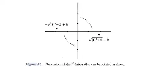
   My first question is, why does $\ell^0 \equiv i \ell_E^0$ imply this counterclockwise rotation. In my understanding, $\ell_E^0$ is the vertical line in the figure, goes from bottom to the top. $\ell^0$ is the horizontal line from left to right. And $\ell_E^0=-i\ell^0$ implies that this rotation is a clockwise rotation from $II$ and $IV$'s region, which cross the poles.

2. On book page 293, the book defined the Wick rotation of time coordinate: $$t\rightarrow -ix^0. \tag{9.44} $$ This seems reasonable to me.

3. If we want to transfer the two-point correlation function from Minkowski space to Euclidean space, which corresponds to eq.(2.59) and (9.48) $$D_F(x-y) \equiv \int \frac{d^4 p}{(2 \pi)^4} \frac{i}{p^2-m^2+i \epsilon} e^{-i p \cdot(x-y)}, \tag{2.59}$$ $$\left\langle\phi\left(x_{E 1}\right) \phi\left(x_{E 2}\right)\right\rangle=\int \frac{d^4 k_E}{(2 \pi)^4} \frac{e^{i k_E \cdot\left(x_{E 1}-x_{E 2}\right)}}{k_E^2+m^2}. \tag{9.48} $$ I have tried to use eq.(6.48) and (9.44) to derive out (9.48) from (2.59), but I find they have a minus sign difference between the time component, in other words, I got: $$\left\langle\phi\left(x_{E 1}\right) \phi\left(x_{E 2}\right)\right\rangle=\int \frac{d^4 k_E}{(2 \pi)^4} \frac{e^{-i k_E^0 \cdot\left(x_{E 1}^0-x_{E 2}^0\right) + i \mathbf{k_E}\cdot \left(\mathbf{x_{E 1}-x_{E 2}}\right)}}{k_E^2+m^2}. $$ So which is correct?

The above three points are my confusion about Wick rotation, could you (Qmechanic) and other people, please elaborate more about this, thanks!

Answer 1

Ref. 1 uses the Minkowski signature convention $(+,-,-,-)$, which is unnatural from the perspective of Wick rotation, cf. e.g. my Phys.SE answer here.

1. E.g. eq. (6.48) then seems to indicate that the Euclidean signature in Ref. 1. is $(-,-,-,-)$. The continuous Wick rotation of the integration contour in quadrant I & III of Fig. 6.1 in Ref. 1 can be viewed as $$\begin{align} \ell^0(\theta)~=~&e^{i\theta}\ell^0_E, \qquad \theta~\in~[0,\frac{\pi}{2}], \qquad \ell^0_E~\in~\mathbb{R},\cr \ell^0(\theta\!=\!0)~=~&\ell^0_E, \qquad \ell^0(\theta\!=\!\frac{\pi}{2})~=~i\ell^0_E=\ell^0_M.\end{align}\tag{6.48}$$ Incidentally, this Wick rotation (6.48) may also be understood in the opposite signature convention, cf. eq. (J) in my Phys.SE answer here. The Wick rotation (6.48) in momentum space works as long as we don't also consider the Wick rotation in spacetime.

2. The arrow in the Wick rotation (9.44) in spacetime should be understood as $$ t_M~=~-i x^0_E, \tag{9.44}$$ cf. my Phys.SE answer here.

3. OP's third question involves a double-Wick-rotation in both spacetime and momentum space, so eq. (6.48) does no longer apply, as also shown by OP's own calculations.

   • Firstly, the Feynman propagator (2.59) in Ref. (1) corresponds (up to a phase factor normalization) to $$ \Delta(x_M\!-\!x^{\prime}_M)~=~ \int\!\frac{d^4 k_{\bullet M}}{(2\pi)^4} \frac{e^{i k_M(x_M-x^{\prime}_M)}}{k^2_M+m^2/\hbar^2 -i\epsilon} \tag{8.11} $$ in Ref. 2 with the opposite signature convention $(-,+,+,+)$.

   • Secondly, eq. (8.11) in Ref. 2 is related to the Euclidian 2-point function (9.48) in Ref. 1 (up to a phase factor normalization), cf. the first part of my Phys.SE answer here, which relies on a compatible Wick rotation convention for both spacetime and momentum space.

References:

1. M.E. Peskin & D.V. Schroeder, An Intro to QFT.

2. M. Srednicki, QFT, 2007; Chapter 71. A prepublication draft PDF file is available here.

Answer 2

The euclidean variabile is on the $x$-axis of the Gauss plane, so the imaginary variable is on the vertical axis. And about the scalar product, you are in Minkowski spacetime, so there is not the minus sign difference between time and space parts if you consider $k_\alpha x^\alpha$ that is $k_0 x^0 + k_i x^i$, but if you consider for example the sum of contravariant components, say $g^{\alpha\beta} k_\alpha x_\alpha$, then it has the form $k_0 x_0 - \sum\limits_i k_i x_i$. Hope it helps a little bit.

P. S. : Wick rotation is really justified once you apply residues theorem, demonstrating that the integrand vanish in the "rotation part" of the closed path

Answer 3

My first question is why $\ell^0 \equiv i \ell_E^0$ imply this counterclockwise rotation.

The integration variable $\ell_E^0$ is supposed to be real. If $\ell_E^0$ runs from $-\infty$ to $\infty$ then the path of integration for $\ell^0=i\ell_E^0$ runs from $-i\infty$ to $i\infty$, which is the vertical line in the figure (y-axis in complex z=x+iy plane).

In my understanding, $\ell_E^0$ is the vertical line in figure, goes from bottom to the top.

No. They want $\ell_E^0$ to be real. So, $i\ell_E^0$ is the vertical line in the figure, which is running from bottom to top as $\ell_E^0$ runs from $-\infty$ to $\infty$.

$\ell^0$ is the horizontal line from left to right.

As $\ell_E^0$ runs from $-\infty$ to $\infty$ it alone would describe the horizontal line from left to right. But we have $\ell^0=i\ell_E^0$. So, in this case, $\ell^0$ alone is not running horizontally from left to right

And $\ell_E^0=-i\ell^0$ implies this rotation is a clockwise rotation from $II$ and $IV$'s region, which cross the poles.

No, the opposite sense of rotation, as shown in the figure. Again, this is because $\ell_E^0$ is real and running from $-\infty$ to $\infty$.

2. On book page 293, the book defined the wick rotation of time coordinate $$t\rightarrow -ix^0 \tag{9.44} $$ this seems reasonable to me.

OK.

3. If we want to transfer the two-point correlation function from Minkowski space to Euclidean space, which correspond to eq.(2.59) and (9.48) $$D_F(x-y) \equiv \int \frac{d^4 p}{(2 \pi)^4} \frac{i}{p^2-m^2+i \epsilon} e^{-i p \cdot(x-y)} \tag{2.59}$$ $$\left\langle\phi\left(x_{E 1}\right) \phi\left(x_{E 2}\right)\right\rangle=\int \frac{d^4 k_E}{(2 \pi)^4} \frac{e^{i k_E \cdot\left(x_{E 1}-x_{E 2}\right)}}{k_E^2+m^2} \tag{9.48} $$

This integral has the poles in exactly the places shown in the figure (i.e., at $\pm\omega_p \mp i\epsilon/\omega_p$). The integration in real momentum-space runs from $p^0=-\infty$ to $p^0=\infty$. So when you change the path you have to integrate up the imaginary axis or you will cross the poles and the answer will be different.

I have tried to use eq.(6.48) and (9.44) to derive out (9.48) from (2.59), but I find their have a minus sign difference between the time component, in other words, I got

$$\left\langle\phi\left(x_{E 1}\right) \phi\left(x_{E 2}\right)\right\rangle=\int \frac{d^4 k_E}{(2 \pi)^4} \frac{e^{-i k_E^0 \cdot\left(x_{E 1}^0-x_{E 2}^0\right) + i \mathbf{k_E}\cdot \left(\mathbf{x_{E 1}-x_{E 2}}\right)}}{k_E^2+m^2} $$ So which is correct.

This is getting fairly close to a "check my work" type of question, which is off-topic for this site. Anyways, in the Euclidean metric you should not have a relative sign between your time and space terms.

As explained above, the Wick rotation is performed as expected and it is a standard procedure for changing the path of integration as is well-known in the field of complex analysis. The path change is valid since the large half-circles "at infinity" can be neglected because of how fast the integrand falls off "at infinity" and because the new path is still circumventing the poles in the same way.

Peskin and Shroder are using the "mostly minus" metric convention. So that: $$ -ip\cdot x = -i(p^0ct - \vec p \cdot \vec x) \;. $$ When we change the path of integration we are now integrating along, for example, the z path: $$ z=i p^0\;, $$ where $p^0$ is real and runs from $-\infty$ to $\infty$. This means we have: $$ -ip\cdot x = -i(-izct - \vec p \cdot \vec x) $$ and, when we make the replacement $ct\to -ix_E^0$ we find: $$ -ip\cdot x = -i(-zx_E^0 - \vec p \cdot \vec x)\;. $$