My expectation is that inherently no such universal algorithm exists.
That said: there are patterns.
I will discuss statics, and classical mechanics.
(For discussion of classical dynamics I refer to an answer I submitted in october 2021, on the subject of Hamilton's stationary action )
I will first discuss the catenary problem.
I start with setting up the differential equation for the catenary, then I will discuss how to construct the corresponding Lagrangian. Then I will discuss how the variational approach finds the catenary
The catenary
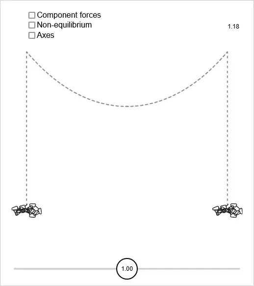
The image shows a hanging chain in a state of force equilibrium.
The image is stylized, the idea is that at the cusps the chain can move freely. Imagine there are frictionless rollers at the cusps.
The length of the vertical sections is set up to provide the amount of tension force that is required for force equilibrium with the length of chain hanging between the cusps. (I use the line integral to compute the length of the chain, and I used the derivative to compute the angle at the cusps.)
(The image is a screenshot of an interactive diagram that is on my own website.)
As we know: the graph of the hyperbolic cosine gives the shape of the hanging chain.
First:
To set up the differential equation for the shape of the catenary.
Since the shape is symmetric it is sufficient to evaluate from the midpoint to the cusp.
The catenary is in force equilibrium at every point along its length. Hence at every point along its length the local tension force is tangent to the local slope.
With:
$T_H$ The horizontal component of the tension
$λ$ The weight per unit of length
$L$ the length of the chain from the midpoint to the x-coordinate.
The weight that has to be supported at coordinate x is given by multiplying the length L with the weight per unit of length: $λL$
The differential equation setup here uses the following property: gravity is acting in the vertical direction therefore there is no gradient in the horizontal component of the tension. That is: the horizontal component of the tension is not a function of the x-coordinate, but constant
In preparation: from midpoint to cusp the slope of the curve increases; the length of chain per unit of x-coordinate increases accordingly. (1.1) gives an expression for dL/dx, which will later be used.
$$ (dL)^2=(dx)^2+(dy)^2 \quad \Leftrightarrow \quad \frac{dL}{dx} = \sqrt{1 + \left(\frac{dy}{dx}\right)^2} \tag{1.1} $$
At every point along the catenary the slope of the curve is equal to the ratio of horizontal tension component and vertical tension component:
$$ \frac{dy}{dx} = \frac{\lambda L}{T_H} \tag{1.2} $$
We need an expression with the derivative of $L$ with respect to $x$, so that (1.1) can be put to use. $T_H$ and $λ$ are constants, so we can treat $λ$/$T_H$ as a constant multiplication factor.
$$ \frac{dy}{dx} = L \frac{\lambda}{T_H} \tag{1.3} $$
Taking the derivative:
$$ \frac{d^2y}{dx^2} = \frac{\lambda}{T_H} \frac{dL}{dx} \tag{1.4} $$
Combining (1.4) and (1.1) allows us to eliminate the quantity dL, arriving at a differential equation that is is purely in terms of the cartesian coordinates $x$ and $y$:
$$ \frac{T_H}{\lambda}\frac{d^2y}{dx^2} = \sqrt{1 + \left(\frac{dy}{dx}\right)^2} \tag{1.5} $$
To simplify the quantity $T_H/\lambda$ is set so a value of 1, so that it can be omitted. (We have the option of putting it back later.)
$$ \frac{d^2y}{dx^2} = \sqrt{1 + \left(\frac{dy}{dx}\right)^2} \tag{1.6} $$
(Thanks to Daniel Rubin for pointing out the following strategy to solve (1.6). Youtube video: The Catenary)
We make the substitution $\tfrac{dy}{dx}=u$, and we square both sides. Squaring both sides introduces an extraneous solution, so at a later stage we must discard that.
$$ \left(\frac{du}{dx}\right)^2 = 1 + u^2 \tag{1.7} $$
Differentiating with respect to $x$ allows the expression to be simplified:
$$ 2\frac{du}{dx}\frac{d^2u}{dx^2} = 2u\frac{du}{dx} \tag{1.8} $$
After dividing by $2\tfrac{du}{dx}$:
$$ \frac{d^2u}{dx^2} = u \tag{1.9} $$
So the solution to the equation is a function with the property that if you differentiate it twice you are back to the original function. That narrows the options down to the hyperbolic sine and the hyperbolic cosine. Checking against the original equation rules out the hyperbolic sine.
(1.10) incorporates the ratio $\tfrac{T_H}{λ}$ such that it satisfies (1.5)
$$ y = \tfrac{T_H}{\lambda} \cosh \left(\tfrac{\lambda}{T_H} x \right) \tag{1.10} $$
Variational approach
Take, as usual, the horizontal axis as the x-coordinate, and the vertical axis as the y-coordinate.
The objective is to find the y-coordinate as a function of the x-coordinate.
Differential approach is that you probe the function by introducing an infinitisimally small increment of the x-coordinate, and you examine how the y-coordinate responds to that.
Variational approach operates at right angles to that.
You probe the function by introducing an infinitisimally small increment, but that increment is increment of the y-coordinate.
The variation of variational calculus is always variation of the other coordinate.
In the case of the catenary:
The variation is variation of height; the y-coordinate
In the case of classical dynamics:
The equation of motion gives position as a function of time. If you plot time coordinate and position coordinate in a cartesian coordinate system: the variation of height that is applied is variation of the coordinate that is at right angles to the time coordinate.
The relation between force equilibrium and potential energy level
The potential energy as a function of position is obtained by evaluating the integral of force with respect to the position coordinate.
That is the definition of potential energy: it is the integral of exerted force with respect to the position coordinate.
In the case of the catenary setup as represented in the image:
When the hanging part sags lower the length of the hanging part increases, and the vertical sections move up by that amount.
We have that the vertical section(s), and the catenary section, are each a repository of potential energy.
When the catenary section sags down the catenary section is doing work, raising the potential energy of the vertical section(s).
When the catenary section is lifted up the vertical section is doing work, raising the potential energy of the catenary section.
To find the equilibrium position you find the shape such that there is no longer any opportunity to do work.
Any shape of the catenary that still has opportunity for conversion of potential energy is not (yet) the shape of lowest possible potential energy. The catenary shape is there when there is no longer opportunity for conversion of potential energy; lowest possible potential energy.
If you probe with an infinitisimally small variation and you find that over that infinitisimally small variation an equal amount of work is done either way: that is the equilibrium point.
Variational approach
The variational approach consists of the following:
You take the derivative with respect to the position coordinate of each of the repositories , and then you identify the point where those derivatives have the same value.
In the case of the catenary: the variational approach takes the derivative of the potential energy with respect to the position coordinate.
As we know: since potential energy is the integral of exerted force with respect to the position coordinate: the derivative of the potential energy with respect to the position coordinate is the force.
Hence the variational approach does the same thing as the differential approach does: the procedure finds the force equilibrium.
As mentioned at the start:
For discussion of classical dynamics I refer to an answer I submitted in october 2021, on the subject of Hamilton's stationary action )
General discussion:
The variational approach takes the derivative with respect to the position coordinate. So: in order to do the same thing as the differential equation the inputs of variational approach must first be converted to the corresponding integral with respect to position coordinate.
That is how variational approach is applied in Statics. You integrate the force with respect to the spatial coordinate, and then - to find the point of lowest possible potential energy - you take the derivative of the potential energy with respect to the position coordinate.
How variational approach is applied in Classical mechanics:
The integral of $F$ (Force) with respect to the position coordinate is the potential energy.
The integral of $ma$ with respect to the position coordinate is $\tfrac{1}{2}mv^2$, kinetic energy. Your objective is to find the trajectory such that the rate of change potential energy is equal to the rate of change of kinetic energy. To identify that point of equal rate of change you take the derivative of the energy with respect to the spatial coordinate.
