Measurement accuracy in quantum mechanics?

Question

Here's some classical background to this thought experiment. Let us first consider a classical scale ruler (called A) of a continuous classical variable. Rulers must be discretised. Let's compare this ruler to one which is 100 times finer (called B) and plot random measurements A = x as a distribution in B. This distribution will come out to be a (slightly smoothed off) rectangle whose width is the interval in A. In order to plot this measurement as a continuous variable, one would therefore naturally represent each measurement using a 'bar graph'. In some sense, every ruler no matter how precise has this uncertainty. However this uncertainty is artificial in that there is classical 'information' about the measurement that the experimenter chooses to ignore.

Now consider the same variable for a quantum wavefunction. The wavefunction is confined to a 1d line and we shall consider how the graph of $\lambda_i$ (eigenvalue of state) on x-axis and $P_i$ (probability) on the y-axis changes. Let's introduce quantum mechanical ruler A, this ruler deliberately scrambles (though this might be difficult to conceive how) classical information about the position so that upon collapse of the wavefunction, the distribution in $\lambda_i$ is a gaussian or random (perhaps a product of these with the original distribution) distribution around the actual measurement $\lambda_a$, which is degenerate in $i$. This can be proven if we introduce a 'perfect' quantum ruler B instantaneously after A and note the distribution in $\lambda_i$.

Now the question is, what is the Hermitian operator of quantum mechanical ruler A? Certainly, if it is simply the original operator discretised by $d\lambda$ then the claim is that the wavefunction collapses into a projection onto the eigenspace (in particular it is a normalised product of a random distribution length $d\lambda$ with the original distribution). However, isn't it more likely for the wavefunction to collapse to something smoother?

The crux of this thought experiment is that all quantum mechanical rulers must in a sense scramble information about the observable. There is no such thing as a perfect ruler. Therefore the corresponding Hermitian operators must be perturbed slightly. The question of what these collapses look like or how they occur can only be answered by introducing better and better quantum mechanical rulers. The question of how sharp this collapse is and what constitutes a perfect ruler has not been answered. This is because the question of what constitutes 'information' about an observable has never been answered. Why is a screen a position ruler, and not a momentum 'ruler'?

Answer 1

As per Emilio Pisanty's nice answer here, a more subtle model of measurement than bare, naive projections (which I reference in this answer) is obtained by considering positive operator-valued measures rather than projection-valued measures as our mechanism for wavefunction "collapse."

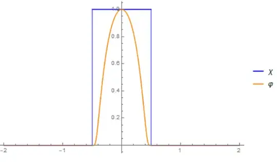
As an example of the latter, imagine a position detector which yields two possible outcomes - that the particle is in the interval $[-a,a]$, or that it is not (of course, this could be generalized to an entire ruler). We then construct the corresponding projection-valued measure via the indicator function $$\chi(x) = \begin{cases}1 & x\in[-a,a]\\ 0 & \text{else}\end{cases}$$ $$\mathbb I = P_\mathrm{in}+P_\mathrm{out} = \int \chi(x) |x\rangle\langle x| \mathrm dx + \int (1-\chi(x))|x\rangle\langle x| \mathrm dx$$

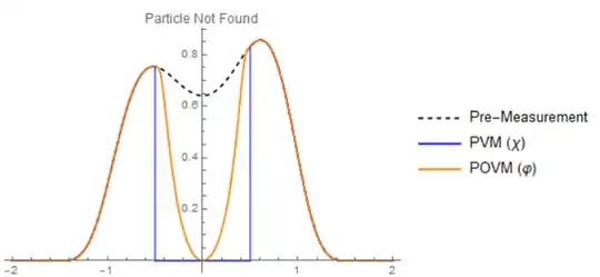
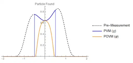
Given a pre-measurement state $|\psi\rangle$, the post-measurement state corresponding to the particle being detected inside $[-a,a]$ is $P_\mathrm{in}|\psi\rangle = \int \chi(x) \psi(x) |x\rangle$, while the post-measurement state corresponding to the particle not being found is $P_\mathrm{out}|\psi\rangle=\int (1-\chi(x))\psi(x)|x\rangle$. The respective probabilities of obtaining these outcomes are $$p_{in/out} = \frac{\Vert P_\mathrm{in/out}|\psi\rangle\Vert^2}{\Vert|\psi\rangle\Vert^2}=\frac{\langle \psi|P_\mathrm{in/out}|\psi\rangle}{\langle \psi|\psi\rangle}$$

As discussed in your question and Emilio's answer above, this is mathematically consistent but raises some thorny issues physically, related to the "clipping" at the edges of $[-a,a]$ where the post-measurement state becomes discontinuous. Therefore, we will swap out our indicator function $\chi$ for a smooth and compactly-supported bump function, $$\varphi(x) = \begin{cases}\exp\left[1-\frac{1}{1-x^2/a^2}\right] & x\in[-a,a]\\ 0 & \text{else} \end{cases}$$ We see once again that

$$\mathbb I = \tilde P_\mathrm{in}+\tilde P_\mathrm{out} = \int \varphi(x) |x\rangle\langle x| \mathrm dx + \int (1-\varphi(x)) |x\rangle\langle x| \mathrm dx$$ $$p_\mathrm{in/out} = \frac{\langle \psi|\tilde P_\mathrm{in/out}|\psi\rangle}{\langle \psi|\psi\rangle}$$

Note that $\tilde P_\mathrm{in/out}$ are no longer projection operators (applying them twice is different from applying them once) because $\varphi^2 \neq \varphi$. This leads to an important difference between POVMs and PVMs - namely, the post-measurement state is not given by $\tilde P_i |\psi\rangle$, but rather $M_i|\psi\rangle$ where $M_i^\dagger M_i = \tilde P_i$. Projection operators are Hermitian and idempotent, so for PVM's this simply reduces to $M_i=P_i$, but for POVMs it does not. In essence, we need to "square root" our $\tilde P_i$'s, and this introduces a new issue - for any choice of $\{M_i\}$s, the set of operators $\{UM_i\}$ produces precisely the same POVM for any unitary $U$.

In other words, the $\tilde P_i$'s which define our POVM do not uniquely define our post-measurement states. They uniquely define our measurement probabilities, but in order to know the post-measurement state we need to make a choice of $\{M_i\}$'s.

Here's the simplest example - let $$M_\mathrm{in} = \int \sqrt{\varphi(x)} |x\rangle\langle x| \mathrm dx$$ $$M_\mathrm{out} = \int \sqrt{1-\varphi(x)} |x\rangle\langle x| \mathrm dx$$

It's easy to see that $M_i^\dagger M_i = \tilde P_i$, and with this choice we have that $$|\psi\rangle_\mathrm{in/out}=M_\mathrm{in/out} |\psi\rangle$$

Unlike before, these post-measurement states are smooth everywhere and no issues with clipping or unphysical post-measurement states arise.

This generalization allows us to model the sensitivity and details of our detector. In this example, the detector registers no "false positives" (i.e. if the detector says it's in the bin $[-a,a]$, then the post-measurement state is entirely within the bin) and is less sensitive near the bin edges. If you choose a gaussian rather than a bump function, the former is no longer true because the support of the gaussian extends over the whole real line.

---

The fact that a POVM does not uniquely define our post-measurement states can be understood from Naimark's theorem, which tells us that any POVM on some Hilbert space $\mathcal H_A$ can be understood as a PVM on a larger space $\mathcal H_A'$. Physically, the idea is that we must couple our system to a model of our measurement device, and the details of this coupling affect the possible post-measurement states of the system being measured.

Two different models of this interaction may yield the same set of probabilities while having completely different post-measurement states, and it is here that we find the physical origin of the ambiguity discussed above. If all we want are the probabilities of various outcomes, then writing down a POVM is sufficient; on the other hand, if we want to know what states the system might be in after the measurement has been performed, we need more details about precisely how the system interacts with the measurement device, which is encoded in a specific choice of $\{M_i\}$.