What is known about the density of states of the Anderson model?

Question

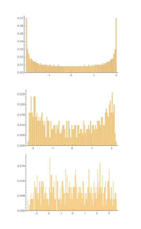
This question was posted a week ago on MathOverflow https://mathoverflow.net/q/369156/

The Anderson Model is given by the random Hamiltonian (as an operator on $l^2(\mathbb{Z}^d)$)

$$ H_\omega = - \Delta + V(\omega) $$ where $V(\omega) \mid x \rangle = \omega(x) \mid x \rangle$ with $\{ \omega(x) \}_{x \in \mathbb{Z}^d}$ independent and uniformly distributed in $[-L, L]$.

It is known for example by Kunz and Soulliard that the spectrum $ \sigma(H_\omega) = [-L, 4d +L ]$. This is also easily verified by simulating finite dimensional approximations. By simulation it is also easy to look at the density of states. Below I have plotted the density of states for $L=0,1,5$ for a $500 \times 500$ approximation. One can see that the high probabilities towards the end of the spectrum wash out. So far this is all numerics, but what is known analytically about this particular density of states?

$L=0,1,5$ for 500x500 approximatio" />

Answer 1

A great (and mathematically rigorous) review on Anderson's model can be found in Aizenman's textbook, Random Operators: Disorder Effects on Quantum Spectra and Dynamics. See CHapter 3 and 4 for discussions/bounds on density of states.

And just a side note, it's actually pretty difficult to numerically verify that $\sigma(H_\omega) = [-L,4d+L]$ as explained by Corollary 4.16 in Aizenman's textbook.