Here we will for fun try to reproduce the first few terms in a perturbative series for the ground state energy $E_0$ of the 1D TISE
$$\begin{align} \hat{H}\psi_0~=~&E_0\psi_0, \cr
H~=~&\frac{p^2}{2}+\frac{\omega^2}{2}q^2+V_{\rm int}(q), \cr
V_{\rm int}(q)~=~&gq^3, \cr
g~=~&\frac{\lambda}{6},\end{align} \tag{A}$$
using an Euclidean path integral in 0+1D
$$\begin{align} e^{W_c[J]/\hbar}~=~&Z[J]\cr
~=~&\int_{q(0)=q(T)}^{\dot{q}(0)=\dot{q}(T)}\!{\cal D}q ~\exp\left\{ \frac{1}{\hbar}\int_{[0,T]}\!dt~(-L_E +J q) \right\} \cr
~=~&\exp\left\{-\frac{1}{\hbar}\int_{[0,T]}\!dt~V_{\rm int}\left(\hbar \frac{\delta}{\delta J}\right) \right\} Z_2[J],\end{align} \tag{B}$$
cf. Refs. 1-3. The Euclidean Lagrangian is
$$\begin{align} L_E~=~&\frac{1}{2}\dot{q}^2+\frac{\omega^2}{2}q^2+V_{\rm int}(q), \cr
q(T)~=~&q(0),\qquad \dot{q}(0)~=~\dot{q}(T), \end{align} \tag{C}$$
with periodic boundary conditions$^1$.
The free quadratic part is the harmonic oscillator (HO)
$$ \begin{align}Z_2[J]&~=~\cr
Z_2[J\!=\!0]&\exp\left\{\frac{1}{2\hbar}\iint_{[0,T]^2}\!dt~dt^{\prime} J(t) \Delta(t,t^{\prime})J(t^{\prime}) \right\}.\end{align} \tag{D}$$
The partition function for the HO can be calculated either via path integrals (e.g. as a functional determinant) or via its definition in statistical physics:
$$\begin{align} Z_2[J\!=\!0]
~=~&{\rm Tr}\left(e^{-\hat{H}(g=0)~T/\hbar}\right)\cr
~=~&\sum_{n\in\mathbb{N}_0}e^{-(n+1/2)\omega T}\cr
~=~&\left(2\sinh\frac{\omega T}{2}\right)^{-1}\cr
~\stackrel{(F)}{=}~&\frac{\sqrt{q}}{1-q}.\end{align} \tag{E}$$
The notation
$$ q~:=~e^{-\omega T}~\in~[0,1[\tag{F}$$
(inspired by the theory of modular forms) should not be confused with the position variable $q$.
The free propagator/Greens function with periodic boundary conditions is
$$ \begin{align} \Delta(t,t^{\prime})
~=~~&\frac{1}{2\omega}\sum_{n\in\mathbb{Z}} e^{-\omega |t-t^{\prime}+nT|}\cr
~\stackrel{|t-t^{\prime}|\leq T}{=}&\frac{1}{2\omega}e^{-\omega |t-t^{\prime}|}+\frac{1}{\omega}\frac{\cosh\omega(t-t^{\prime})}{e^{\omega T}-1}\cr
~=~~&\frac{1}{2\omega}\left(\frac{e^{-\omega|t-t^{\prime}|}}{1-e^{-\omega T}} +\frac{e^{\omega|t-t^{\prime}|}}{e^{\omega T}-1}\right)\cr
~=~~&\frac{\cosh\omega\left(|t-t^{\prime}|-\frac{T}{2}\right)}{2\omega\sinh\frac{\omega T}{2}}, \cr
\Delta(0,0)~=~&\frac{1}{2\omega}\coth\frac{\omega T}{2}~\stackrel{(F)}{=}~\frac{1+q}{1-q},\cr
\left(-\frac{d^2}{dt^2}+\omega^2\right)\Delta(t,t^{\prime})
~=~~&\delta(t\!-\!t^{\prime}+T\mathbb{Z})~=:~{\rm III}_T(t\!-\!t^{\prime}),\end{align}\tag{G}$$
where ${\rm III}_T$ is the Dirac comb/shah function. Eq. (G) becomes in the $T\to\infty$ limit
$$ \begin{align} \Delta(t,t^{\prime})~=~&\frac{1}{2\omega}e^{-\omega |t-t^{\prime}|}, \cr
\Delta(0,0)~=~&\frac{1}{2\omega},\cr
\left(-\frac{d^2}{dt^2}+\omega^2\right)\Delta(t,t^{\prime})
~=~&\delta(t\!-\!t^{\prime}).\end{align}\tag{H}$$
The main idea is to use the fact that the ground state energy can be inferred from the connected vacuum bubbles$^2$
$$ \frac{1}{\hbar}W_c[J\!=\!0]~\stackrel{(J)}{\sim}~ -E_0(g) T\quad\text{for}\quad T\to\infty.\tag{I}$$
Here we are using the linked-cluster theorem$^3$
$$\begin{align} e^{W_c[J=0]/\hbar} ~=~&Z[J\!=\!0]
~=~{\rm Tr}\left(e^{-\hat{H}T/\hbar}\right)\cr
~=~&\sum_{n\in\mathbb{N}_0}e^{-E_n(g)T/\hbar} \end{align} \tag{J}$$
(The free connected vacuum part $\frac{1}{\hbar}W_{c,2}[J\!=\!0]$ in eq. (E) is often graphically represented by a self-loop $\bigcirc$, cf. footnote 1 of my Phys.SE answer here. We stress that $\bigcirc$ is not an ordinary perturbative Feynman diagram.)
The Feynman rule for the cubic vertex is
$$ -\frac{\lambda}{\hbar}\int_{[0,T]}\!dt. \tag{K}$$
The unperturbed zero-mode energy for the HO is the well-known
$$E_0(g\!=\!0)~=~E_0^{(0)}~=~\frac{\hbar\omega}{2},\tag{L} $$
cf. eq. (E). Set $\hbar=1=\omega$ to compare with OP's eq. (3).
There are two 2-loop vacuum bubbles: the dumbbell diagram $O\!\!-\!\!O$ and the sunset diagram $\theta$ with symmetry factor $S=8$ and $S=12$, respectively, cf. Fig. 1.
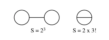
$\uparrow$ Fig. 1. (From Ref. 4.) The two 2-loop vacuum bubbles: the dumbbell diagram $O\!\!-\!\!O$ and the sunset diagram $\theta$.
They make up the 2nd-order contribution
$$ g^2E_0^{(2)}~=~-\frac{11\hbar^2 g^2}{8\omega^4} \tag{M} $$
to the ground state energy $E_0(g)$, cf. OP's eq. (3) & Ref. 5.
Proof of eq. (M): The dumbbell Feynman diagram $O\!\!-\!\!O$ is$^4$
$$ \begin{align}
\frac{(-\lambda/\hbar)^2}{8} \hbar^3&
\iint_{[0,T]^2}\!dt~dt^{\prime}
~\Delta(t,t)\Delta(t,t^{\prime})\Delta(t^{\prime},t^{\prime})\cr
~\stackrel{(G)}{=}~&\frac{(-\lambda/\hbar)^2}{8} \left(\frac{\hbar}{2\omega}\right)^3 \iint_{[0,T]^2}\!dt~dt^{\prime}
\left(\frac{e^{-\omega |t-t^{\prime}|}}{1-e^{-\omega T}} +\frac{e^{\omega |t-t^{\prime}|}}{e^{\omega T}-1}\right)
\coth^2\frac{\omega T}{2}\cr
~=~& \frac{\hbar\lambda^2}{32\omega^4}T\coth^2\frac{\omega T}{2}\cr
~=~& \frac{9\hbar g^2}{8\omega^4}T\coth^2\frac{\omega T}{2}.\end{align}\tag{N}$$
The sunset Feynman diagram $\theta$ is
$$ \begin{align}
\frac{(-\lambda/\hbar)^2}{12} \hbar^3& \iint_{[0,T]^2}\!dt~dt^{\prime}
\Delta(t,t^{\prime})^3\cr
~\stackrel{(G)}{=}~& \frac{(-\lambda/\hbar)^2}{12} \left(\frac{\hbar}{2\omega}\right)^3 \iint_{[0,T]^2}\!dt~dt^{\prime}
\left(\frac{e^{-\omega |t-t^{\prime}|}}{1-e^{-\omega T}} +\frac{e^{\omega |t-t^{\prime}|}}{e^{\omega T}-1}\right)^3\cr
~=~& \frac{\hbar\lambda^2}{144 \omega^4}T\left(1+\frac{3}{\sinh^2\frac{\omega T}{2}}\right)\cr
~=~& \frac{\hbar g^2}{4\omega^4}T\left(1+\frac{3}{\sinh^2\frac{\omega T}{2}}\right).\end{align}\tag{O}$$
The sum of the dumbbell and sunset diagrams becomes$^3$
$$
\frac{\hbar g^2}{8\omega^4}T\left(11+\frac{15}{\sinh^2\frac{\omega T}{2}}\right)
~=~ \frac{11\hbar g^2}{8\omega^4}T + {\cal O}(T^0)
.\tag{P}$$
To obtain eq. (M) compare eqs. (I) and (P).
$\Box$
Five 3-loop vacuum bubbles make up the 4th-order contribution, cf. Fig. 2.
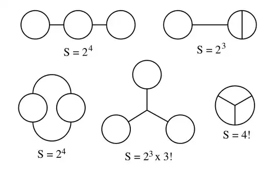
$\uparrow$ Fig. 2. (From Ref. 4.) The five 3-loop vacuum bubbles.
It is in principle possible to calculate to any order by drawing Feynman diagrams. An $n$-loop-integral is analytically doable by breaking the integration region $[0,T]^n$ into $n$-simplexes.
References:
M. Marino, Lectures on non-perturbative effects in large $N$ gauge theories, matrix models and strings, arXiv:1206.6272; section 3.1.
R. Rattazzi, The Path Integral approach to Quantum Mechanics, Lecture Notes for Quantum Mechanics IV, 2009; subsection 2.3.6.
R. MacKenzie. Path Integral Methods and Applications, arXiv:quant-ph/0004090, section 6.
M. Srednicki, QFT, 2007; figures 9.1 + 9.2. A prepublication draft PDF file is available here.
I. Gahramanov & K. Tezgin, A resurgence analysis for cubic and quartic anharmonic potentials, arXiv:1608.08119, eqs. (3.1) + (3.2).
--
$^1$ We need 2 boundary conditions since the EOM is a 2nd-order ODE. It is natural to assume that the trajectories $t\mapsto q(t)$ are differentiable.
$^2$ On one hand, in the frequency space a connected Feynman diagram with $n$ external legs is of the form
$${\cal M}(k^0_1,\ldots, k^0_n)\delta(k^0_1\!+\!\ldots\!+\!k^0_n)\tag{Q}$$
due to time translation invariance. Moreover ${\cal M}(k^0_1,\ldots, k^0_n)$ is finite in QM, cf. e.g. my Phys.SE answer here. In particular each vacuum bubble is proportional to the time period $\delta(0)\sim T$. On the other hand, in the time domain the propagator is bounded
$$|\Delta(t,t^{\prime})|~\leq~ \Delta(0,0)~=~\frac{1}{2\omega}\coth\frac{\omega T}{2},\tag{R}$$
so Feynman diagrams in the time domain are finite if the time region $[0,T]$ is compact.
$^3$ It is in principle possible to derive all the energy-levels
$$E_n(g)~=~\underbrace{E_n^{(0)}}_{=(n+1/2)\hbar\omega}+ g\underbrace{E_n^{(1)}}_{=0} + g^2E_n^{(2)} +g^3\underbrace{E_n^{(3)}}_{=0} +{\cal O}(g^4)\tag{S}$$
from the identity (J)
$$\begin{align}\sum_{n\in\mathbb{N}_0}&e^{-E_n(g)T/\hbar} \cr
~\stackrel{(J)+(P)}{=}&\left(2\sinh\frac{\omega T}{2}\right)^{-1}\exp\left\{\frac{\hbar g^2}{8\omega^4}T\left(11+\frac{15}{\sinh^2\frac{\omega T}{2}}\right)+{\cal O}(g^4)\right\}\cr
~=~&\sqrt{q}\left(\sum_{k\in\mathbb{N}_0}q^k\right)
\left\{1+\frac{\hbar g^2}{8\omega^4}T\left(11+ 60\sum_{\ell\in\mathbb{N}_0}\ell q^{\ell}\right)+{\cal O}(g^4)\right\}
\end{align}\tag{T}$$
as a power series in $g$ and $q$. It's a fun exercise to check that the identity (T) agrees with the 2nd-order correction from standard Rayleigh–Schrödinger (RS) perturbation theory
$$ \begin{align}
g^2 E_n^{(2)}
~=~& \sum_{k\neq n} \frac{|\langle k^{(0)}| \hat{V}_{\rm int}| n^{(0)}\rangle |^2}{E_n^{(0)}-E_k^{(0)}}\cr
~=~& \frac{\hbar^2g^2}{8\omega^4} \left(\frac{n(n-1)(n-2)}{3} + 9n^3 -9(n+1)^3 -\frac{(n+3)(n+2)(n+1)}{3} \right)\cr
~=~& -\frac{\hbar^2g^2}{8\omega^4} \left(30n^2 +30n +11\right),
\end{align} \tag{U}$$
as it should.
$^4$ It is straightforward to check that
$$\begin{align} \iint_{[0,T]^2}\!dt~dt^{\prime}e^{-\omega |t-t^{\prime}|}
~=~& 2\int_0^T \!dt\int_0^t\!dt^{\prime}e^{-\omega (t-t^{\prime})}\cr
~=~&\frac{2}{\omega}\left(T -\frac{1-e^{-\omega T}}{\omega} \right)\cr
~=~&\frac{2T}{\omega} + {\cal O}(T^0),\end{align} \tag{V}$$
$$\iint_{[0,T]^2}\!dt~dt^{\prime}~\Delta(t,t^{\prime})
~\stackrel{(G)}{=}~\iint_{[0,T]^2}\!dt~dt^{\prime}~\frac{\cosh\omega\left(|t-t^{\prime}|-\frac{T}{2}\right)}{2\omega\sinh\frac{\omega T}{2}}
~\stackrel{(V)}{=}~\frac{T}{\omega^2},\tag{W}$$
$$\iint_{[0,T]^2}\!dt~dt^{\prime}~\Delta(t,t^{\prime})^2 ~\stackrel{(G)+(V)}{=}~\frac{T}{4\omega^2}\left(\frac{1}{\omega}\coth\frac{\omega T}{2}+\frac{T}{2\sinh^2\frac{\omega T}{2}}\right),\tag{X}$$
$$\iint_{[0,T]^2}\!dt~dt^{\prime}~\Delta(t,t^{\prime})^3 ~\stackrel{(G)+(V)}{=}~\frac{T}{12\omega^4}\left(1+\frac{3}{\sinh^2\frac{\omega T}{2}}\right).\tag{Y}$$