How the classical trajectory arise in the classical limit of quantum harmonic oscillator?

Question

The quantum harmonic oscillator $H=\frac{p^2}{2m}+\frac{1}{2}m\omega^2 x^2$ has energies $E_n=\hbar\omega(n+1/2)$, so to achieve "classical" energies $n$ must be very large.

My question is: how does appear the classical behaviour of a point mass in this potential, as energy increases? Classically, a point mass has exactly the position $x(t)=a\cos(\omega t)$, suggesting that the wavefuntion $\psi$ verifies that its square $|\psi(x,t)|^2\cong 0$ everywhere except near $x=a\cos(\omega t)$.

In this hyperphysics page appears that probability is well approximated. Taking the wave function $\psi_n$ corresponding to the energy $E_n$, with large $n$:

\begin{equation} \psi_n(x,t)=e^{-iE_nt/\hbar}\psi_n(x,0) \end{equation}

It yields:

\begin{equation} |\psi_n(x,t)|^2=|\psi_n(x,0)|^2 \end{equation}

For large energies, this quantum probability density approaches the classical probability density. But that is different than saying that $|\psi(x,t)|^2\cong 0$ everywhere except near $x=a\cos(\omega t)$!

I know that the mean value $\langle x\rangle$ does follow a sinusoidal "motion" when there is a linear combination of two or more energy eigenstates, but that is different because $\langle x\rangle$ is related to measuring $x$ a lot of times and then computing the mean value, while classically only one measure is needed. I mean, if $|\psi(x,t)|^2$ were $\cong 0$ everywhere except near $x=a\cos(\omega t)$, then, with only one measure of $x$, the result would be (in the vast majority of cases) $\cong a\cos(\omega t)$.

So, more realistically, let's consider a linear combination of states $\psi_n$ (a lot of states) all with high "classical" energies:

\begin{equation} \psi(x,t)=\sum_{n\ \text{large}}\psi_n(x,t) \end{equation}

Does $|\psi(x,t)|^2\cong 0$ everywhere except near $x=a\cos(\omega t)$, recovering the classical motion?

Answer 1

Does $|\psi(x,t)|^2\cong 0$ everywhere except near $x=a\cos(\omega t)$, recovering the classical motion?

Yes, this is exactly the logic of Schroedinger's minimal uncertainty wavepacket (coherent state) as linked by @ZeroTheHero in his good answer. Namely, for the parameters specified in the WP article, $$ |\psi(x,t)|^2=\sqrt{\frac{m\omega}{\pi\hbar} } e^{-\frac{m\omega}{\hbar}\left(x- \langle \hat{x}(t) \rangle \right)^2 } , $$ where $\langle \hat{x}(t) \rangle =a \cos(\omega t) $, for some choice of phase specifying the origin of time-keeping. So you see the width of this probability Gaussian goes like $\sqrt \hbar$ (where $\hbar\sim 10^{-30}$ times the action of a freshman lab classical oscillator), squishing it to the $\delta$-function you visualize in your final phase of the question. Behold the oscillating Gaussian of the WP article!

Even though this answers your question, I'd like to dwell on the quite reasonable first phase of your question, which often confuses readers only by dint of language and picture, not physics and the counterintuitive peculiarities of QM! A stationary state for a given large n you are considering will provide a stationary probability distribution versus x, ably discussed in this question; so, for large n, the QM distribution morphs to the time averaged classical distribution of your hyperlink. Where did the time average come from? What is a stationary classical distribution?

The stationary classical distribution is but the ensemble/average of all classical trajectory phases/origins-of-time. Just as a specific classical trajectory is represented by a point rotating uniformly on a phase-space plot, a sum/average of all phases of such yields a thick palisade, indeed, a cookie cutter, of all such points on a circle (corresponding to a constant energy circular shell, ~ $p^2 + x^2$, where all masses, frequencies, etc... are absorbed in the units). The entire ensemble of trajectories share the same energy, merely differing in phase, or start time. Integrating over all p s will yield the U-shaped classical probability distribution $1/\sqrt{a^2-x^2}$ of your hyperlink. So when you compare apples with apples there is a chance (below).

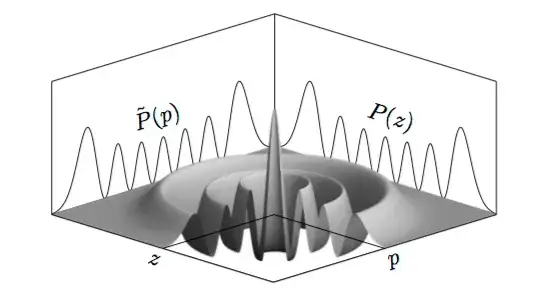
Now, you might object that QM abhors xs and ps in the same breath, but this is not so. An equivalent, alternative formulation of QM in phase space works, and the quasi-probability distribution in phase space grows with n to supplant the classical cookie cutter for suitably scaled phase-space variables accomodating the large n and small $\hbar$. Integrating w.r.t. p, indeed approximates the classical U-shaped distribution quite well, exactly as you set up to anticipate!

Here is a cartoon of the n=6 Wigner distribution with its p and x projections (where the conjugate variable is integrated over; they use z here instead of x), already beginning to look like the U. Recall the oscillator is completely x-p symmetric.