1

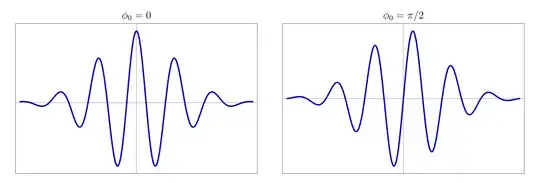
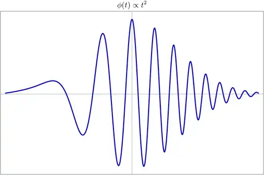
An ultrashort laser pulse can usually be written as a product of a time-varying envelope $A(t)$ and a periodic function with angular frequency $\omega$

$$E(t)=A(t)\cos(\omega t+\phi(t)+\phi_0)$$

Where $\phi(t)$ is temporal phase and $\phi_0$ the absolute phase .

(I found this kind of expressions in the book Ultrafast Nonlinear Optics, by Reid, and in the PhD thesis Ultrashort pulse characterization in amplitude and phase from the IR to the XUV.)(25th page)

My question is why this is so? What is the basis? I cannot understand the importance of $\phi(t)$ and $\phi_0$.

Pictorial approach is welcomed.

Icchyamoy
  • 442

2 Answers2

3

The two quantities play rather different roles here.

  • $\phi_0$ is known as the carrier-envelope phase (sometimes carrier-envelope offset) or CEP, and it governs the shape of the pulse. If your pulse is relatively long (more than, say, ten effective cycles or so), then you don't expect the CEP to matter much, unless your experiment is strongly susceptible to the shape of the pulse, in which case you need to look very carefully at exactly how you're modelling your pulse envelope $A(t)$.

    The CEP's role kicks in for short pulses, and it determines whether the peak of the envelope coincides with a peak of the carrier (and if so, in which direction), or with a node. Pictures say it best, I think:

    Mathematica graphics

  • The time-dependent phase $\phi(t)$ is normally introduced to add some amount of chirp to the pulse. The lowest meaningful dependence is quadratic about the maximum of the envelope (because a linear variation can just be incorporated into $\omega$), and roughly speaking it changes the local frequency at different points in the pulse:

    Chirped pulses have a local frequency which goes either up or down during the pulse. Saying anything more about chirp is a bit harder because it depends on the context, but here are some general aspects:

    • During the amplification stage, pulse chirp is a crucial tool, because it enables us to make the pulse longer while retaining coherence between the different spectral components. The technique is known as chirped pulse amplification, and it works by making the pulses longer via a chirp, so that they are less intense and therefore safe to amplify, and then you re-compress by undoing the chirp.

    • On the other hand, if your pulse is on the infrared, odds are that you're not interested in sending it into your interaction chamber with any amount of chirp, because it makes the pulse longer (thus messing with your temporal resolution) and less intense. Part of the problem here is that pretty much all transmissive optics (and some reflective optics, too) are dispersive, which means that they introduce chirp; that therefore means that folks in the lab end up spending a good amount of time measuring, controlling, and cutting down on that chirp.

    • Things change a bit if your pulse is not the IR driving pulse but an attosecond XUV pulse produced during high-order harmonic generation, because here you have much less control over the harmonic emission. Here you still want to have as little chirp as possible, because chirp always makes the pulse longer than its Fourier-transform limit and you normally want as short an XUV pulse as you can possibly get, but unfortunately most HHG-produced attosecond pulses have an intrinsic chirp, often called the attochirp. (Yeah, I know, we're great at naming things. At least this post hasn't called in the animal acronyms.)

      The origin of this attochirp comes from the good old energy-time mapping from the semiclassical model of HHG: different electrons are tunnel-ionized at different times, so they come back to the ion at different recollision times and with different energies:

      Image source: Nature Photon 8, 187–194 (2014)

      This gets directly mapped onto the emitted spectrum: if you're catching the long trajectories, then higher frequencies will come in earlier, and vice versa for the short trajectories. That's not great, and there's a good deal of work going on to try and roll that chirp back - or you might just accept it and roll with chirped XUV pulses if they're already short enough for whatever it is you want to do with them.

Mathematica graphics through Import["http://halirutan.github.io/Mathematica-SE-Tools/decode.m"]["https://i.sstatic.net/y7c4E.png"]

Emilio Pisanty
  • 137,480
1

I think that the explanation follows from this quote (on the next page in the document you linked, that is the page numbered '11' but which is the 26th page in the document):

If the temporal phase $\phi(t)$ changes non-linearly with time, the oscillation period of the electric field also becomes a function of time. In other words, the frequency changes with time during the pulse, which is called a chirp

In other words - ultrashort pulses often have a variable frequency (chirp). However, there is some value in describing a "center frequency" $\omega_0$ that is fixed; while it would in principle be possible to describe the frequency at a later time as $\omega(t)$, this leaves the tricky problem of describing the phase of the wave (if you vary the frequency with time, then the offset of phase with time will also have to change). You can get around this problem by just using a time-varying phase - because that essentially encompasses time-varying frequency. The converse is not true: time varying frequency cannot be described without also including a time-varying phase.

Floris
  • 119,981