What are the electromagnetic fields of a photon?

Question

I'm looking for expressions for the electromagnetic fields (preferably $E$ and $B$) of a typical photon which is localised in space to some extent (i.e. I'm not interested in the infinite plane wave solution of Maxwell's equations).

Answer 1

The short answer is $\vec E=\vec B=0$. Strange as it may sound, this is only one of the numerous counter intuitive facts of the quantum realm. But first let me try to clarify, without going into mathematical details, the context within which these equalities should be interpreted.

Perhaps one of the easiest ways to approach the quantum nature of the electromagnetic field in the vacuum is to study the field in a perfectly conducting cavity.

Classically, such cavity supports distinct, countably infinite modes, each with its own specific frequency and spacial profile. The electromagnetic field attributed to each mode is completely defined by the shape of the cavity, up to a multiplying constant, which represents the energy contained in each mode.

In the quantum field approach, the values of the energy each mode contains are quantized and equally spaced, given by the expression $$E = \hbar\omega (n+1),$$ with $n$ being equal to "the degree of excitation", or number of photons of each mode.

The number of photons is an observable physical quantity related to the operator $\hat{N}$, but in quantum optics, as well as in single particle quantum mechanics, not all operators of all observable quantities commute. In particular $\hat{N}$ does not commute with $ \hat{\mathbf{E}}$ and $\hat{\mathbf{B}}$, the operators of the electric and magnetic field respectively. In other words, one cannot know the number of photons and the value of the electric field simultaneously.

When the cavity is in an eigenstate of $\hat{N}$, which is usually called a number state, or Fock state, the expectation value of the electric field operator and the magnetic field operator is equal to zero. This is what the expression at the beginning implies. On the other hand, the fluctuations are proportional to the classical values of the field and increase with increasing numbers of photons.

States where the expectation value of the electric field takes its classical value, are called coherent states and are considered to be the ones closest resembling classical light more closely. In such states, the exact number of photons is not known.

To rephrase my initial statement, it is impossible to attribute some field value to a photon, except in the sense of the expectation value in a 1-photon-number state, where it is always equal to zero.

Answer 2

Light, the classical electromagnetic field , is built up/emerges from a large number of photons, not in a simple manner.

Photons are elementary particles and therefore can only be described within a quantum mechanical framework. They have a wave-function that obeys the potential form of Maxwell's equations turned into operators which operate on the photon wave function. In this link a path is shown of how the classical wave emerges from the quantum state. Hand-waving my understanding of this: a photon, in addition to its spin, has information connected with A, the electromagnetic potential which information builds up the corresponding potential of the classical wave, and thus the macroscopically observed electric and magnetic fields of light.

There exists also this preprint.

Properties of six-component electromagnetic field solutions of a matrix form of the Maxwell equations, analogous to the four-component solutions of the Dirac equation, are described. It is shown that the six-component equation, including sources, is invariant under Lorentz transformations. Complete sets of eigenfunctions of the Hamiltonian for the electromagnetic fields, which may be interpreted as photon wave functions, are given both for plane waves and for angular-momentum eigenstates

In this preprint there is explicit an E and B field in the expression of the photon wavefunction.( One should always keep in mind that the wave function squared gives a probability distribution).

Answer 3

The answer is: you can't ask. That is, the question is counter-factual, in the quantum-mechanical sense.

In quantum electrodynamics, your goal is to include electromagnetism into the same type of quantum mechanics that you use things like the motion of an electron around the atom or a particle undergoing diffraction in a double-slit experiment. In quantum mechanics, you take the dynamical quantity of interest (say, the position of an electron around an atom) and you build wavefunctions on top of that dynamical quantity: $$ \begin{array}{c} \text{classical mechanics}\\ x(t) \end{array} \ \mapsto\ \begin{array}{c} \text{quantum mechanics}\\ \psi(x,t) \end{array} $$ This means that you can no longer speak about "the" value of the particle; instead, if you decide to measure the position of the particle at a time $t$, then you can talk about the distribution of possible values and their probabilities (given by $|\psi(x,t)|^2$), as well as things as the average value, the width of the distribution, and so on.

In quantum electrodynamics, your variables of interest are essentially the electric field amplitudes* $E(t)$, so you do the same thing: you knock out the "having-a-value-ness" of that dynamical variable, and you change it for a wavefunction: $$ \begin{array}{c} \text{classical electrodynamics}\\ E(t) \end{array} \ \mapsto\ \begin{array}{c} \text{quantum electrodynamics}\\ \psi(E,t) \end{array} $$ This means, therefore, that you can no longer speak about "the" value of the electric field; it has become an operator and no longer has a value. Instead, you have some distribution.

Given some reasonable assumptions, the probability distribution for the amplitude of a given mode (i.e. some travelling or standing wave) when the field is in a one-photon state looks more or less like this:

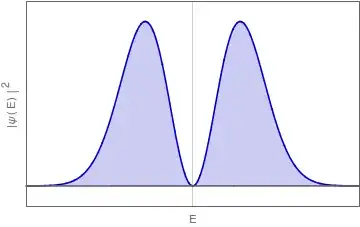
In this state, you can have a reasonably good idea of the value of the square of the amplitude, but most importantly you have no information about the phase of the oscillations of the node. Among other things, this means that the average value of the field from that mode at any given point will be zero.

There's plenty of additional subtleties to be had, but this is a reasonable starting point.

---

^{This obviously hides plenty of nuance, but the essentials stand. In reality, your dynamical variables are the amplitudes of given modes, i.e. $E(t)$ is the amplitude of some standing or travelling wave. There's also trouble in dealing with gauges and so on, but once you've done all that it still looks much the same.}

^{Mathematica code for the image through Import["http://halirutan.github.io/Mathematica-SE-Tools/decode.m"]["https://i.sstatic.net/334QY.png"].}

Answer 4

As you already noted, photons are not physical - as they correspond to infinite wave train solutions.

When most people refer to photons, they probably refer to those blips which individually hit a detector screen. I'm not sure what those actually are, since they're not infinitely sharp but have smear patterns - like Gaussian smears.

What you're asking for - and what better corresponds to what you see on a detector screen - is something more localized. These are better described with the aid of coherent states.

In quantum field theory, the components of the electromagnetic field are q-numbers, rather than c-numbers: they don't all commute with each other and their commutators are actually singular when non-zero (i.e. delta functions), as is the case generally with fields. The expectation values of these q-numbers in any state are zero, because of conservation laws, so they can only represent quantum fluctuations (i.e. the expectation values of quadratic combinations of the field components are generally non-zero). The actual q-numbers are linear combinations (integrals, actually) of the annihilation operators, one set for each wave-number 3-vector.

In contrast, coherent states are eigenstates of the creation and annihilation operators and produce more sensible results, when taking their expectation values. Here is one reference that discusses this in more detail and shows a decomposition of the q-number field (which the expectation value in a coherent state can be directly read off of):

S.J. van Enk, "Coherent states, beam splitters and photons" (Lecture Notes)
https://pages.uoregon.edu/svanenk/solutions/NotesBS.pdf

As an exercise, you may want to write out the electromagnetic field components, like in part 7 in the reference and apply it to a coherent state (like those described in part 6) and determine whether it satisfies Maxwell's equations in vacuuo or not. The result should be the same as the mode expansion for the electromagnetic field, with the creation and annilation operators replaced by function-conjugate function pairs.

This is still an infinite wave train, but you may superpose coherent states to obtain wave packets localized in space (e.g. Gaussian wave packets). Then the issue of dispersion over time arises.

Another reference that discusses two photon coherent states is:

Horace P. Yuen, "Two-photon coherent states of the radiation field", Physical Review A, Volume 13, Number 6, 1976 June
https://journals.aps.org/pra/pdf/10.1103/PhysRevA.13.2226

which is apparently, at the time of writing, freely accessible.

The Wikipedia article on Coherent States:

https://en.wikipedia.org/wiki/Coherent_state

illustrates both the electric field of a given coherent state and its quantum fluctuation at different photon numbers. The quantum fluctuation for the total field - as a ratio to the field itself - decreases with increasing photon number, as expected; and the field comes to more and more resemble the wave train given classically.

There is a folklore result that asserts that "photons cannot be localized". In reality, the actual result falls in the same category as the statement "the sphere cannot be uniformly coordinatized". In symplectic geometry, in both classical physics and in quantized form, there do exist position operators for photons, with a minor qualification. The symplectic geometry for photons falls under the category of what might be called "helical luxons"; i.e. luxons whose angular momentum lie on an axis parallel to their momentum, with its helicity being an invariant.

The Darboux Theorem ensures that all symplectic geometries can be represented locally in a set of conjugate (p,q) coordinate pairs. Like spin 0 luxons (and also spin 0 tardions and even spin 0 tachyons) they can be represented by 3 coordinate pairs - which is in contrast to the spin non-zero tardions, which have 4 (the 4th, which when quantized, corresponds to the m coordinate in the usual representation of angular momentum). A position operator for helical luxons involves 3 sets of complementary coordinate pairs that cover most - but not all - of the underlying symplectic geometry and - when quantized - satisfies the same Heisenberg relations as particle coordinates do. The situation is analogous to how the magnetic monopole is coordinatized (which is described in Section 8.2 "Magnetic Monopoles" in LNP 188 "Gauge Symmetries and Fibre Bundles"). There is a dependency on a choice of a reference vector, much in the same way that spherical coordinates depend on a choice of an axis, and along that axis the coordinates become singular in a similar way. The choice of reference vector is a "geometrical gauge".

An example where the position operator is used is:

Hawton, Margaret; Baylis, William E. "Angular momentum and the geometrical gauge of localized photon states" https://www.osti.gov/biblio/20650498-angular-momentum-geometrical-gauge-localized-photon-states

Overall, the issue of photon localization seems to be a topic of active discussion in the literature, but it is as new to me as it is to you. A brief search, for instance, uncovers the following:

Ayman F. Abouraddy, Giovanni Di Giuseppe, Demetrios N. Christodoulides, and Bahaa E. A. Saleh
"Anderson localization and colocalization of spatially entangled photons"
Rapid Communications, Physical Review A 86, 040302(R) (2012)

while Anderson localization is discussed more fully here:

https://en.wikipedia.org/wiki/Anderson_localization

Beyond this, and on the more general issue of localization, I can't say much.