I found expressions for the solution, and I write them below. With the help of a software I checked that they really are the solutions, I'm 100% sure: they solve the differential equation
\begin{equation*}
m \ddot{x} + c \dot{x} + kx= F \cos(\omega t )
\end{equation*}
and satisfy the initial conditions (initial position $x_0$ and initial speed $v_0$). But obviously the job isn't done, for the simple reason that the solution I write are really ugly: it must be possible to write this formulas in a better way. We should do it for aesthetic reasons, obouvisly, but also to make them more easy to handle, and so more useful. The beautiful work I did with the not forced case (see the question) allow users to find easily the equation of motion of the particle (exploring limiting cases too is simple). I tried to do the same with the forced case but I wave the white flag, I can't do it (I won't work more about this problem). I hope someone will do. Anyway I write out the complete solution (althoung in this ugly form).
Case 1: $c=2\sqrt{m k}$
\begin{equation*}
x(t) = \frac{e^{-\frac{c t}{2 m}} \left( A+B+C \right) }{B_2}
\end{equation*}
where
\begin{equation*}
\begin{split}
&A= \left( A_1 + A_2 \right) F \\
&B= \left( B_1 + B_2 \right) x_0 \\
&C= 2 m (m \omega^2 + k)^2 t v_0 \\
&A_1= 2 m e^{\frac{c t}{2m}} \left( c \omega \sin \left( \omega t\right) -m \omega^2 \cos\left( \omega t\right) +k \cos\left( \omega t\right) \right) \\
&A_2 = -c \left( m \omega^2 + k \right) t+2 m^2 \omega^2-2 k m \\
&B_1 = c {\left( m \omega^2+k\right) }^2 t \\
&B_2 = 2 m ( m \omega^2 + k )^2
\end{split}
\end{equation*}
Case 2: $c>2\sqrt{m k}$
\begin{equation*}
x(t) = \frac{e^{-\frac{U}{2 m}-\frac{c t}{2 m}} \left( x_0 W \left( e^{\frac{U}{m}} +1\right) +\sqrt{c^2-4 k m} \left( F L +v_0 E+x_0 D\right) +F G\right) }{2W}
\end{equation*}
where
\begin{equation*}
\begin{split}
& L = \left( c m \omega^2+c k\right) e^{\frac{U}{m}}-c m \omega^2-c k \\
& D = cV \left( 1-e^{\frac{U}{m}} \right) \\
& E = 2mV \left( 1-e^{\frac{U}{m}} \right) \\
& G = K e^{\frac{U}{m}}+K+G_2+G_1 \\
& K = O \left( m \omega^2-k\right) \\
& W = O V \\
& G_1 = 2 c O \omega \sin\left( \omega t\right) Z \\
& G_2 = -2 O \left( m \omega^2-k\right) \cos \left( \omega t\right) Z \\
& O = 4 k m-c^2 \\
& Z = e^{\frac{U}{2 m}+\frac{c t}{2 m}} \\
& U = \sqrt{c^2-4 k m} t \\
& V = {m}^2 \omega^{4}-2 k m \omega^2+c^2 \omega^2+{k}^2
\end{split}
\end{equation*}
Case 3: $c<2\sqrt{m k}$
\begin{equation*}
x(t) = \frac{e^{-\frac{c t}{2 m}} \left( S+R+\sqrt{4 k m-c^2} \left( Q+P \right) +N \right) }{\sqrt{4 k m-c^2} \left( m^2 \omega^4+\left( c^2-2 k m \right) \omega^2+k^2 \right) }
\end{equation*}
where
\begin{equation*}
\begin{split}
P=&\left( c \omega e^{\frac{c t}{2 m}} \sin \left( \omega t \right) +\left( k-m \omega^2 \right) e^{\frac{c t}{2 m}} \cos \left( \omega t \right) +\left( m \omega^2-k \right) \cos \left( \frac{\sqrt{4 k m-c^2} t}{2 m} \right) \right) F \\
Q=&\left( m^2 \omega^4+\left( c^2-2 k m \right) \omega^2+k^2 \right) \cos \left( \frac{\sqrt{4 k m-c^2} t}{2 m} \right) x_0 \\
R=&-c\left( m \omega^2 + k \right) \sin \left( \frac{\sqrt{4 k m-c^2} t}{2 m} \right) F \\
S=&c \left( m^2 \omega^4+\left( c^2-2 k m \right) \omega^2+ k^2 \right) \sin \left( \frac{\sqrt{4 k m-c^2} t}{2 m} \right) x_0 \\
N=& m \left( 2 m^2 \omega^4+\left( 2 c^2 -4 k m \right) \omega^2+2 k^2 \right) \sin \left( \frac{\sqrt{4 k m-c^2} t}{2 m} \right) v_0
\end{split}
\end{equation*}
An example
This work look a mess but it isn't: it allow to get elegant solution for physical problems (provided you have a computer to help you, if expressions won't be simplified, as I hope someone will do, calculus by hands will be prohibitive!). But let's consider a concrete example. Suppose we have exactly (I don't transcribe units, simply suppose they are consistent) $c=1$, $k=2$, $\omega = 3$, $F=4$, $x_0 = 5$, $v_0 = 6$, $m=2{.}5$ we get this equation of motion (we are in the third case)
\begin{equation*}
\begin{split} x(t)=&
\frac{59703 e^{-\frac{t}{5}} \sin \left( \frac{\sqrt{19} t}{5} \right) }{1717 \sqrt{19}}+\frac{8913 e^{-\frac{t}{5}} \cos \left( \frac{\sqrt{19} t}{5} \right) }{1717}+\\ & \frac{48 \sin \left( 3 t \right) }{1717}-\frac{328 \cos \left( 3 t \right) }{1717}
\end{split}
\end{equation*}
We see that when $t$ is big (after transient) the motion is approximately given by
\begin{equation*}
x(t) = -\frac{8 }{\sqrt{1717}} \cos \left( 3 t+\tan^{-1} \left( \frac{6}{41}\right) \right)
\end{equation*}
I obtained this from $x(t) = \frac{48 \sin \left( 3 t \right) }{1717}-\frac{328 \cos \left( 3 t \right) }{1717}$, but looking the formula $x(t)$ of case 3 we can write a general formula for this motion after transient: I find strange that it is completely independent by initial condition:
\begin{equation*}
x_{at}(t) = \frac{\left( c \omega \sin \left( \omega t\right) +\left( k-m {\omega}^2\right) \cos \left( \omega t\right) \right) F}{m^2 {\omega}^{4}+\left( {c}^2 -2 k m\right) {\omega}^2 +{k}^2 }
\end{equation*}
But we know exactly all the motion, not only this limiting state: here I plot $x=x(t)$
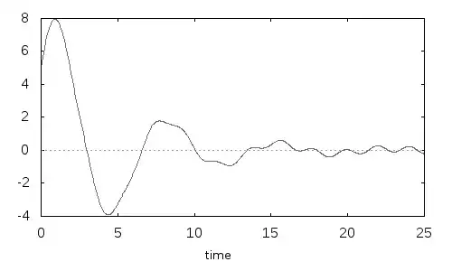
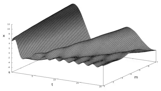
If we wait in doing the final substitution $m=2{.}5$, we can get the two variable function that tell us how varies the motion if we vary the mass $m$ (the previous graph is the section of this below at $m=2{.}5$ and with $t$ until 25):
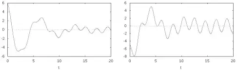
With derivative of $x(t)$ we can find speed and acceleration as function of $t$:
In short, knowing analytic solution allow us to find exactly any kind of information: for example we can find that after 8 seconds (or unit of time you are using) the position is about $1{.}727745920373746$ and after 15 seconds acceleration is $0{.}3102092667738571$, or more precisely
\begin{equation*}
\frac{72 \left( 41 \cos \left( 45\right) - 6 \sin \left( 45\right) \right) }{1717} -
\frac{24 \left( 6133 \sin \left( 3 \sqrt{19}\right) +2332 \sqrt{19} \cos \left( 3 \sqrt{19}\right) \right) }{8585 \sqrt{19} e^3 }
\end{equation*}
We can also find exactly other kind of information, for example we can estimate (necessarily numerically in this case, but only because we have transcendental equations: errors are very small and we can estimate them) that the particle meet the $x=0$ position, for the first time, when $t \approx 2{.}9818321933898$ (and for the first time it is at rest when $t=0{.}90687408051175$). I defy anyone to find better data using a numerical ODE solver: with my formulas I can find exact position at any time, while solving ODE numerically give more approximate data than find the value of a formula (and it is not easy estimate the error). Of course all this digit have no sense in a real physical problem (physical constant and conditions are not exactly know, linear law for friction is only a rough approximation) but I feel that exact analytic solution of a model (a physical model with all its limits, like every other one) is very gratifying (what about the artificial but beautiful problem we can find in electrostatic for example?). I hope someone will write my exact but ugly solution, in the right way (it MUST exists a RIGHT way to write it).