I'll show to you "how this is the case", "how this works", but this needs time. This is a very interesting question and I'm sorry to see that books divide in two set: basic one that simply jump the problem (maybe mentioning it or reporting formula saying that calculations are boring, while they are exciting); and advanced ones, that obviously deal with a such important problem, but they solve everything with few symbols using such hard mathematics that they are difficult to be understood by less capable readers (here I am). I find that the best compromise is, as always, Griffiths (from which I take most of this answer). But for once I want criticize his book too. He put the reader in front of the traumatizing divergence of a matrix, without prepare him to handle a such object. That's why I'll put in this answer a section named "Alternative divergence theorem". Here I will always use cartesian coordinates, simply I ascertain that this is the simplest way to see why there is a momentum density of the electromagnetic field and to calculate how much it is. These calculations are long, but if the reader trust me he/she will be gratified.
Momentum current density
It is necessary to introduce the concept of momentum current density. Like current density $\mathbf{J}$ is a vector such that $\mathbf{J} \cdot d\mathbf{a} dt$ gives the amount of charge that pass through $d\mathbf{a}$
in interval $t \to t+dt$; momentum current density is a matrix such that ${\sf{M}} \cdot d\mathbf{a} dt$ gives the amount of momentum that flow through $d\mathbf{a}$ in interval $t \to t+dt$. Charge is a scalar so current density is a vector, but momentum is a vector so it sounds reasonable introduce a matrix to describe its current density (the dot product with a vector gives a vector). In this definition I don't say if I have to do ${\sf{M}} \cdot d\mathbf{a}$ or $d\mathbf{a} \cdot {\sf{M}}$, but this is the same: we will see that in cartesian coordinate momentum current density is a symmetric matrix.
An interesting way to describe the momentum conservation
Let's suppose that inside volume $V$ are moving charged particles in electromagnetic field (not necessarily all given by the charge themselves).
Let's be $d\mathbf{p}$ the change, during the time $dt$, of momentum of these bodies into the volume $V$. If we can write this equation,
\begin{equation}
\frac{d\mathbf{p}}{dt} = - \frac{d}{dt} \int_V \mathbf{C} d \tau - \oint_S {{\sf{D}}} \cdot d \mathbf{a}
\end{equation}
then the only reasonable interpretation is that $\mathbf{C}$ is momentum density of the field and ${\sf{D}}$ is the momentum current density. In fact in this way the equation above says that change of field momentum in interval $t \to t+dt$ inside the volume (i.e. $d \left( \int_V \mathbf{C} d \tau \right) $) is the opposite of variation of momentum of bodies (i.e. $d\mathbf{p}$) minus the field momentum that flowed out through the surface $S$ (i.e. $ \oint_S {{\sf{D}}} \cdot d \mathbf{a} dt $). We are excluding the possibility that bodies cross through surface $S$ in time $dt$, otherwise we should generalize the equation, but we don't need to do that if we are interested to evaluate the momentum of electromagnetic field in the easier way. Take your time to reflect about this equation and these considerations, and see how reasonable they are. Then go on.
Poynting vector and Maxwell tensor definition
Later we will use the vector we define here (introduced by John Henry Poynting in 1884)
\begin{equation}
\mathbf{S} = \frac{\mathbf{E} \times \mathbf{B}}{\mu_0}
\end{equation}
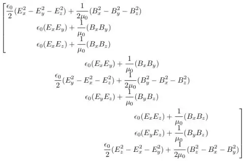
Let me introduce this matrix, at the moment it can sound a mess but later you will see that we introduce this to avoid a mess and express the theorem in an elegant way. Maxwell tensor ${\sf{T}}$ is described by
\begin{equation}
T_{ij} = \epsilon_0 \left( E_i E_j - \frac{1}{2} \delta_{ij} E^2 \right) +\frac{1}{\mu_0} \left( B_i B_j - \frac{1}{2} \delta_{ij} B^2 \right)
\end{equation}
where index $i$ and $j$ refers to three coordinates $x$, $y$ and $z$ (so that tensor has in total 9 components: all possible combinations $T_{xx}$, $T_{xy}$, $T_{xz}$, $T_{yx}$, etc.) and $\delta_{ij}$ is Kronecker delta.
Explicitly we could write (note that to obtain this below we have to substitute field squared in the definition whit sum of squared components)
Alternative divergence theorem
Given a symmetric matrix field ${\sf{M}}$, defined into volume $V$ surrounded by surface $S$, we have
\begin{equation}
\int_V (\nabla \cdot {\sf{M}}) d \tau = \oint_S {\sf{M}} \cdot d \mathbf{a}
\end{equation}
By matrix field we mean an analogous to vector field, but with matrices (each element is a function of $(x,y,z,t)$). The analogy with ordinary divergence theorem is strong (note that $\nabla \cdot$ low by one the dimension of the object to which we apply it). On the left we do a volume integral of products between a vector field and infinitesimal volumes, on the right we do a surface integral of products between a matrix field and infinitesimal surface vectors. In both sides we have an infinite sum of infinitesimal vectors: a finite vector.
Proof of alternative divergence theorem
The proof of this alternative divergence theorem is similar to the one of ordinary divergence theorem. Let's suppose for simplicity that volume $V$ is the parallelepiped $(a<x<b, c<y<d, e<z<f)$. The flux of matrix field ${\sf{M}}$ through the face orthogonal to $x$ axis is
\begin{equation}
\int_e^f \int_c^d {\sf{M}} (a,y,z) \cdot
\begin{bmatrix}
-dydz \\ 0 \\ 0
\end{bmatrix}
+ \int_e^f \int_c^d {\sf{M}} (b,y,z) \cdot
\begin{bmatrix}
dydz \\ 0 \\ 0
\end{bmatrix}
\end{equation}
where we used $\mathbf{\hat{x}} dy dz$ as a column vector (here "hat" mean versor). If $\mathbf{M}_1 (x,y,z)$ is the vector field we get taking first column of matrix ${\sf{M}}$, we can write the flux through the two surfaces in this way
\begin{equation}
\int_e^f \int_c^d [ \mathbf{M}_1 (b,y,z) - \mathbf{M}_1 (a,y,z) ] dydz
\end{equation}
Integrand is a vector that can be written in this way
\begin{equation}
\begin{bmatrix}
M_{xx} (b,y,z) - M_{xx} (a,y,z) \\ M_{yx} (b,y,z) - M_{yx} (a,y,z) \\ M_{zx} (b,y,z) - M_{zx} (a,y,z)
\end{bmatrix}
\end{equation}
And exploiting fundamental theorem of calculus we can write
\begin{equation}
\begin{bmatrix}
\int_a^b \frac{\partial M_{xx} (x,y,z) }{\partial x} dx \\ \int_a^b \frac{\partial M_{yx} (x,y,z) }{\partial x} dx \\ \int_a^b \frac{\partial M_{zx} (x,y,z) }{\partial x} dx
\end{bmatrix}
\end{equation}
Which is $\int_a^b \frac{\partial \mathbf{M}_1}{\partial x} dx $. By substituting we see that flux through two surface can be written
$\int_V \frac{\partial \mathbf{M}_1}{\partial x} dV$. Similarly we can found the flux through other couples of side: the total flux through the parallelepiped is
\begin{equation}
\int_V \left( \frac{\partial \mathbf{M}_1}{\partial x} + \frac{\partial \mathbf{M}_2}{\partial y} + \frac{\partial \mathbf{M}_3}{\partial z} \right) dV
\end{equation}
To end the proof we only have to show that the integrand is equal to the vector we symbolically wrote as $\nabla \cdot {\sf{M}}$. That is, we have to show that
\begin{equation}
\frac{\partial \mathbf{M}_1}{\partial x} + \frac{\partial \mathbf{M}_2}{\partial y} + \frac{\partial \mathbf{M}_3}{\partial z} =
\begin{bmatrix} \displaystyle
\frac{\partial}{\partial x} & \displaystyle
\frac{\partial}{\partial y} & \displaystyle
\frac{\partial}{\partial z}
\end{bmatrix}
\left[
\begin{array}{c|c|c}
& & \\
\displaystyle \mathbf{M}_1 &
\displaystyle \mathbf{M}_2 &
\displaystyle \mathbf{M}_3 \\
& & \\
\end{array}
\right]
\end{equation}
At first glance this looks wrong, but ${\sf{M}}$ is symmetric by hypothesis so the equation works. If you are skeptical about this conclusion, here the proof. In left member we have the sum of three vectors:
\begin{equation}
\left[
\frac{\partial M_{xx}}{\partial x} +
\frac{\partial M_{xy}}{\partial y} +
\frac{\partial M_{xz}}{\partial z} ,
\frac{\partial M_{yx}}{\partial x} +
\frac{\partial M_{yy}}{\partial y} +
\frac{\partial M_{yz}}{\partial z} ,
\frac{\partial M_{zx}}{\partial x} +
\frac{\partial M_{zy}}{\partial y} +
\frac{\partial M_{zz}}{\partial z}
\right]
\end{equation}
while in second member we have the product between a vector (like we do in ordinary vector analysis, it is useful use the symbolism of treating $\nabla$ as a vector) and a matrix:
\begin{equation}
\left[
\frac{\partial M_{xx}}{\partial x} +
\frac{\partial M_{yx}}{\partial y} +
\frac{\partial M_{zx}}{\partial z} ,
\frac{\partial M_{xy}}{\partial x} +
\frac{\partial M_{yy}}{\partial y} +
\frac{\partial M_{zy}}{\partial z} ,
\frac{\partial M_{xz}}{\partial x} +
\frac{\partial M_{yz}}{\partial y} +
\frac{\partial M_{zz}}{\partial z}
\right]
\end{equation}
if matrix is symmetric ($M_{ij}=M_{ji}$) these two expressions are the same. This show that the previous equation is an identity and the proof is ended.
The calculus of electromagnetic field momentum
The electromagnetic force that acts on charges in volume $V$ is
\begin{equation}
\mathbf{F} = \int_V (\mathbf{E} + \mathbf{u} \times \mathbf{B}) \rho d \tau = \int_V ( \rho \mathbf{E} + \mathbf{J} \times \mathbf{B} ) d \tau
\end{equation}
the force per unit volume is
\begin{equation}
\mathbf{f} = \rho \mathbf{E} + \mathbf{J} \times \mathbf{B}
\end{equation}
Exploiting Maxwell equations, it is possible eliminate sources in favor of field. I'll show to you how to do it now. Using first and last Maxwell equation we have
\begin{equation}
\mathbf{f} = \epsilon_0 ( \nabla \cdot \mathbf{E} ) \mathbf{E} + \left( \frac{1}{\mu_0} \nabla \times \mathbf{B} - \epsilon_0 \frac{\partial \mathbf{E}}{\partial t} \right) \times \mathbf{B}
\end{equation}
Now,
\begin{equation}
\frac{\partial }{\partial t} (\mathbf{E} \times \mathbf{B}) =
\left( \frac{\partial \mathbf{E} }{\partial t} \times \mathbf{B} \right) +
\left( \mathbf{E} \times \frac{\partial \mathbf{B} }{\partial t} \right)
\end{equation}
So by exploiting Faraday law we can rearrange in this way
\begin{equation}
\frac{\partial \mathbf{E} }{\partial t} \times \mathbf{B} =
\frac{\partial }{\partial t} (\mathbf{E} \times \mathbf{B}) +
\mathbf{E} \times (\nabla \times \mathbf{E})
\end{equation}
Substituting we have
\begin{equation}
\mathbf{f} = \epsilon_0 \left[
(\nabla \cdot \mathbf{E}) \mathbf{E} - \mathbf{E} \times (\nabla \times \mathbf{E})
\right]
-\frac{1}{\mu_0} \left[ \mathbf{B} \times (\nabla \times \mathbf{B}) \right]
- \epsilon_0 \frac{\partial}{\partial t} (\mathbf{E} \times \mathbf{B})
\end{equation}
Right for make things more symmetrical we can throw in a term $\frac{1}{\mu_0} (\nabla \cdot \mathbf{B})\mathbf{B}$ (it's the same: magnetic field is solenoidal). Now note that applying to the same vector $\mathbf{A}$ the vector identity
\begin{equation}
\nabla (\mathbf{A} \cdot \mathbf{B}) = \mathbf{A} \times (\nabla \times \mathbf{B}) +
\mathbf{B} \times (\nabla \times \mathbf{A}) + ( \mathbf{A} \cdot \nabla )\mathbf{B} + ( \mathbf{B} \cdot \nabla )\mathbf{A}
\end{equation}
will allow us to write
\begin{equation}
- \mathbf{A} \times (\nabla \times \mathbf{A}) = - \frac{1}{2} \nabla (A^2) + (\mathbf{A} \cdot \nabla)\mathbf{A}
\end{equation}
All this allow us to write previous equation in this way
\begin{equation}
\begin{split}
\mathbf{f} = & \epsilon_0 \left[ (\nabla \cdot \mathbf{E}) \mathbf{E} + (\mathbf{E} \cdot \nabla ) \mathbf{E} \right]
- \frac{1}{\mu_0} \left[ (\nabla \cdot \mathbf{B}) \mathbf{B} + (\mathbf{B} \cdot \nabla ) \mathbf{B} \right] \\
& - \frac{1}{2} \nabla \left( \epsilon_0 E^2 + \frac{1}{\mu_0} B^2 \right) - \epsilon_0 \frac{\partial}{\partial t} (\mathbf{E} \times \mathbf{B})
\end{split}
\end{equation}
Despite symmetries, this expression is ugly. Beauty reigns in fundamental law of nature so it must be possible write the equation in a better and clarifier way. It comes to our rescue Maxwell tensor we wrote before and the idea to use the operator $\nabla$ like if it were a vector. Doing scalar product between $\nabla$ and Maxwell tensor we get the second member of the equation written above (less than term with time derivative)
\begin{equation}
\begin{split}
\nabla \cdot {\sf{T}} = & \epsilon_0 \left[ (\nabla \cdot \mathbf{E}) \mathbf{E} + (\mathbf{E} \cdot \nabla ) \mathbf{E} \right]
- \frac{1}{\mu_0} \left[ (\nabla \cdot \mathbf{B}) \mathbf{B} + (\mathbf{B} \cdot \nabla ) \mathbf{B} \right] \\
& - \frac{1}{2} \nabla \left( \epsilon_0 E^2 + \frac{1}{\mu_0} B^2 \right)
\end{split}
\end{equation}
Let's check that this is true: we will be careful on the only $x$ coordinate (for symmetrical reasons other coordinates will work). The $x$ coordinate of the second member of the above equation is
\begin{equation}
\begin{split}
& \epsilon_0 \left[
\left( \frac{\partial E_x}{\partial x} + \frac{\partial E_y}{\partial y} + \frac{\partial E_z}{\partial z} \right) E_x +
E_x \frac{\partial E_x}{\partial x} + E_y \frac{\partial E_x}{\partial y} + E_z \frac{\partial E_x}{\partial z}
\right] \\
& + \frac{1}{\mu_0} \left[ \left( \frac{\partial B_x}{\partial x} + \frac{\partial B_y}{\partial y} + \frac{\partial B_z}{\partial z} \right) B_x +
B_x \frac{\partial B_x}{\partial x} + B_y \frac{\partial B_x}{\partial y} + B_z \frac{\partial B_x}{\partial z}
\right] \\
& - \frac{\epsilon_0}{2} \frac{\partial (E_x^2 + E_y^2 + E_z^2)}{\partial x} -
\frac{1}{2 \mu_0} \frac{\partial (B_x^2 + B_y^2 + B_z^2)}{\partial x}
\end{split}
\end{equation}
While the $x$ coordinate of the first member (i.e. the "scalar product" between $\nabla$ and the first column of Maxwell tensor is)
\begin{equation}
\begin{split}
& \frac{\epsilon_0}{2} \frac{\partial (E_x^2 - E_y^2 - E_z^2)}{\partial x} +
\frac{1}{2 \mu_0} \frac{\partial (B_x^2 - B_y^2 - B_z^2)}{\partial x} \\
& + \epsilon_0 \frac{ \partial ( E_x E_y)}{\partial y} + \frac{1}{\mu_0} \frac{ \partial ( B_x B_y)}{\partial y}
- \epsilon_0 \frac{ \partial ( E_x E_z)}{\partial z} + \frac{1}{\mu_0} \frac{ \partial ( B_x B_z)}{\partial z}
\end{split}
\end{equation}
Reader can easily check that the two terms are equal (for simplicity, because of the symmetry we can concentrate on only one field, for example $E$).
Now we are ready to write the "ugly" equation in a beautiful and compact way:
\begin{equation}
\mathbf{f} = - \epsilon_0 \mu_0 \frac{\partial \mathbf{S}}{\partial t} + \nabla \cdot {\sf{T}}
\end{equation}
where we used Poynting vector too. Exploiting $c=\frac{1}{\sqrt{\epsilon_0 \mu_0}}$ and integrating over volume we have
\begin{equation}
\frac{d\mathbf{p}}{dt} = - \frac{d}{dt} \int_V \frac{\mathbf{S}}{c^2} d \tau +\oint_S {\sf{T}} \cdot d \mathbf{a}
\end{equation}
where we exploited the "Alternative divergence theorem". Now come back to what I wrote in the section "An interesting way to describe the momentum conservation", and reflect: the proof is ended:
- Momentum density: $\frac{\mathbf{S}}{c^2}$
- Momentum current density: $ - {\sf{T}}$
Why Maxwell tensor is not defined with inverted sign? Probably this is due to an unfortunate historical convention. If we want express field momentum as a function of fields we have obviously
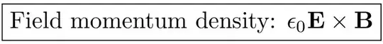 This can be exploited to show that for electromagnetic waves we have $E=pc$ (it is not a case that this is the same link between energy and momentum we have for extreme relativistic particles).
A final comment
Note that what we found suffers from abstraction and give problems: this momentum theorem (like Poynting theorem too) is general, not only for electromagnetic wave: we didn't any special hypothesis about the nature of the field (the only one being that the field obey to Maxwell equations). This lead to very interesting (but also very complicated!) problems related to hidden momentum. As we often see in physics, each time you solve a problem you are in front of harder problems and of strange (and so, interesting) point of reflection on the big puzzle.

