If you purchase a \$100 \space \mathrm{MHz}\$ oscilloscope with the intention of observing a \$100 \space \mathrm{MHz}\$ signal, you will encounter significant measurement error.
The bandwidth \$BW\$, in \$\mathrm{Hz}\$, of your oscilloscope determines the Amplitude Error, as there will be attenuation as the frequency increases, which becomes more significant at the point of \$-3 \space \mathrm{dB}\$ (corner frequency \$\omega_c\$ in \$\mathrm{rad/s}\$). If you are interested only in in the the high frequency side, you can model it rougly as a simple first order system (remebering that the bandwidth stuff refers to analog part of scope):
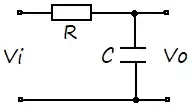
$$\frac{V_o(\omega)}{V_i(\omega)}= \frac{1/j \omega C}{1/j\omega C+R}= \frac{1}{1+j\omega RC}$$
As
$$ RC=\frac{1}{\omega_c}=\frac{1}{2 \pi BW} \qquad (1)$$
the magnitude of that transfer function, as function of frequency \$f = \frac{\omega}{2\pi}\$, in \$\mathrm{Hz}\$, is given by:
$$ \left | \frac{V_o(f)}{V_i(f)} \right | = \frac{1}{\sqrt{1 + \left ( \frac{f}{BW} \right )^2}} \qquad \lt 1 $$
Also:
$$ \left | V_o(f) \right | = \frac{1}{\sqrt{1 + \left ( \frac{f}{BW} \right )^2}} \space \left | V_i(f) \right | \qquad (2)$$
The definition of Amplitude Error is:
$$\text{Amplitude Error (%)}= 100 \left (1- \left | \frac{V_o(f)} {V_i(f} \right | \right )$$
Or:
$$
\boxed
{
\text{Amplitude Error (%)}= 100 \left (1- \frac{1}{\sqrt{1 + \left (
\frac{f}{BW} \right )^2}} \right )
}
$$
If you prefer in a plot:
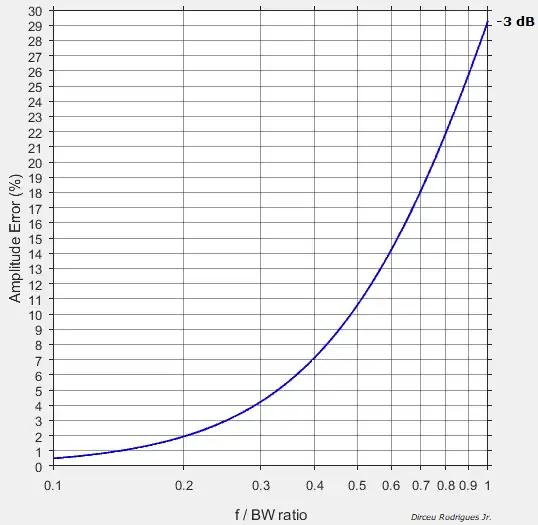
So, if you put sinewave with amplitude \$ 1 \space \mathrm{V}\$ and frequency \$100 \space \mathrm{MHz}\$ as input in a \$100 \space \mathrm{MHz}\$ (\$BW\$) oscilloscope, the Amplitude Error error will be \$29.3 \space \% \$. Also, using \$(2)\$, the voltage \$V_o\$ will be read as aprox. \$0.707 \space \mathrm{V}\$. On the other hand, with a \$500 \space \mathrm{MHz}\$ scope, the Amplitude Error will be aprox. \$ 1.94 \%\$ (or \$ V_o= 0.98 \space \mathrm{V}\$).
In summary: A \$100 \space \mathrm{MHz}\$ scope will have up aprox. \$30 \%\$ error at \$100 \space \mathrm{MHz}\$. To keep errors below the \$3 \%\$, the maximum signal bandwidth that can be measured is about \$30 \%\$ of \$100 \space \mathrm{MHz}\$, or \$30 \space \mathrm{ MHz}\$. In a different way: In order to accurately measure a \$100 \space \mathrm{MHz}\$ signal (below \$3 \%\$ error), you need at least \$300 \space \mathrm{MHz}\$ of bandwidth.
Another consideration is with respect to the rise time of the signal to be measured (which is the time taken by a signal to change from a specified low value to a specified high value, typically from \$10 \%\$ to \$90 \%\$). You can have a rise time of \$10 \space \mathrm{ns}\$ on a "square" signal with a frequency of either \$10 \space \mathrm{Hz}\$ or \$1 \space \mathrm{MHz}\$. In other words, it is the ability to follow this rise time that identifies the quality of the measurement system, not the frequency alone.
A common expression relating the rise time \$tr\$, in seconds, with the bandwith \$BW\$ in \$\mathrm{Hz}\$, is:
$$BW = \frac{0.35}{tr}$$
That expression can be easily obtained considering that circuit in the beginning of this post, along \$(1)\$ and the equation for capacitor charging (from \$10 \%\$ to \$90 \%\$). So, a \$100 \space \mathrm{MHz}\$ oscilloscope has a rise time of \$3.5 \space \mathrm{ns}\$ and a \$500 \space \mathrm{MHz}\$ one, a rise time of \$1.75 \space \mathrm{ns}\$.
Through the Central Limit Theorem, it follows that whenever you have a measurement system formed by others non interacting cascaded sub-systems (one after the other), free from overshoot in their step-responses, each with its own rise time \$tr_1\$, \$tr_2\$, ... and \$tr_n\$, the rise observed time from input to output \$t_r\$ is given by:
$$tr = \sqrt{tr_1^2 + tr_2^2 + \text{...} + tr_n^2}$$
If \$tr_s\$ and \$tr_p\$ are the rise time for the scope and the probe, respectively, then the equation for System Bandwidth in your reference can be obtained as follows:
$$tr = \sqrt{tr_s^2 + tr_p^2} $$
$$\frac{1}{tr} = \frac{1}{\sqrt{tr_s^2+tr_p^2}}$$
$$\frac{BW}{0.35}=\frac{1}{\sqrt{tr_s^2+tr_p^2}}$$
$$BW = \frac{1}{\frac{1}{0.35}\sqrt{tr_s^2+tr_p^2} }$$
$$BW=\frac{1}{\sqrt{\left ( \frac{tr_s}{0.35} \right )^2+ \left ( \frac{tr_p}{0.35} \right )^2}}$$
$$BW=\frac{1}{\sqrt{\left ( \frac{1}{BW_s} \right )^2+ \left ( \frac{1}{BW_p} \right )^2}}$$
Where \$BW\$, \$BW_s\$ and \$BW_p\$ are the system, scope and probe bandwidths, respectively.
Therefore, the response is yes, that expression you have mentioned and associated calculations make sense. But, I believe that the most important is to keep your error lower as possible (remember the rule of \$3 \%\$).
Finally, in a note from Fluke, there is an alternative approach considering the harmonic content in your signal:
Perhaps an even better, and much more conservative, approach is to
consider the stated bandwidth to be that of a fifth harmonic of the
frequency you want to measure. A fifth harmonic, likely present in a
typical pulse, might begin to become attenuated at the
stated bandwidth. That would indicate that we can rely on a 500 MHz
bandwidth oscilloscope to show a full and undistorted picture of the
input at about 100 MHz, maintaining good fidelity of the signal you're
trying to measure.
Using this criteria, a measurement system with \$500 \space \mathrm{MHz}\$ bandwidth is suggested to capture the fifth harmonic of a \$100 \space \mathrm{MHz}\$ square wave.


