To keep the transfer function 2nd order, \$C_4\$ needs to be ignored. No harm in doing so. (It's there to keep the opamp from oscillating at high frequency and doesn't really serve another purpose here.)
What I find is that the critical frequency is, as you already know, \$\omega_{_0}=\frac1{\sqrt{L_2\,C_1}}\$ or \$f_{_0}=\frac1{2\pi\,\sqrt{L_2\,C_1}}\$.
So nothing new there.
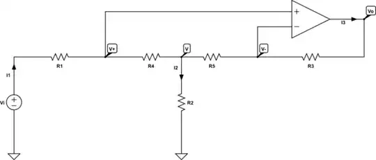
Analysis starts with assigning \$V_x\$ to the wiper point of the potentiometer and then splitting up the potentiometer into two resistor values based upon the wiper position, \$p\$. The following shows how to do it with SymPy/Sage/Python (freely available):
rx1 = p*r1                                      # left side pot R
rx2 = (1-p)*r1                                  # right side pot R
ep = Eq( vp/r2 + vp/rx1,vi/r2 + vx/rx1 )        # (+) opamp node KCL
em = Eq( vm/rx2 + vm/r5, vx/rx2 + vo/r5 )       # (-) opamp node KCL
ex = Eq( vx/rx1 + vx/rx2 + vx/(s*l2+1/s/c1), vp/rx1 + vm/rx2 ) # Vx KCL
eo = Eq( vo/r5, io + vm/r5 )                    # opamp output node KCL
answer = solve( [ep, em, ex, eo, Eq(vm,vp)], [vm, vp, vo, io, vx] )
tf = tf2( an2[vo] / vi )
{
 omega: 1/(sqrt(c1)*sqrt(l2)),
 zeta: sqrt(c1)*(-p**2*r1/2 + p*r1/2 - p*r2/2 + r2/2)/sqrt(l2),
 P: [{A: 1,                                               N: 2},
     {A: p*(p*r1 - r1 - r5)/(p**2*r1 - p*r1 + p*r2 - r2), N: 1},
     {A: 1,                                               N: 0}]
}
(tf2 is a function I wrote some time ago. I can provide it, if needed.)
This is an all-pass filter, so it has all three components:
$$\begin{align*}
H\left(s\right)&=\underbrace{\overbrace{\left[1\vphantom{\frac{\left(1-p\right)R_1-R_5}{\left(1-p\right)R_1+\left(\frac1{p}-1\right)R_2}}\right]}^{\text{gain}}\cdot\frac{\left(\frac{s}{\omega_{_0}}\right)^2}{\left(\frac{s}{\omega_{_0}}\right)^2+\frac1{Q}\left(\frac{s}{\omega_{_0}}\right)+1}}_{\text{high-pass}}
\\\\
& +\underbrace{\overbrace{\left[\frac{\left(1-p\right)\cdot R_1-R_5}{\left(1-p\right)\cdot R_1+\left(\frac1{p}-1\right)\cdot R_2}\right]}^{\text{gain}}\cdot\frac{\frac1{Q}\left(\frac{s}{\omega_{_0}}\right)}{\left(\frac{s}{\omega_{_0}}\right)^2+\frac1{Q}\left(\frac{s}{\omega_{_0}}\right)+1}}_{\text{band-pass}}
\\\\
&+\underbrace{\overbrace{\left[1\vphantom{\frac{\left(1-p\right) R_1-R_5}{\left(1-p\right)R_1+\left(\frac1{p}-1\right)R_2}}\right]}^{\text{gain}}\cdot\frac{1}{\left(\frac{s}{\omega_{_0}}\right)^2+\frac1{Q}\left(\frac{s}{\omega_{_0}}\right)+1}}_{\text{low-pass}}
\end{align*}$$
Where \$0 \le p \le 1\$ is the potentiometer position with 0 being all the way to the left and 1 being all the way to the right.
What I write below assumes the resistor values you provided. There is enough information here that you can alter those values to see how it impacts things. But I'm not going to complicate what I write by discussing how you might want to change those values, as well. I'll leave that part to you. At least there's info to use in considering how they impact the inductor to capacitor ratios. (They do.)
The midband (where you set \$f_{_0}\$) will have a relative gain of about \$2\$ with \$p\approx 0.888\$ or 88.8% towards the right and a relative gain of about \$\frac12\$ with \$p\approx 0.112\$ or 11.2%. Outside the range between those two positions things start to go rapidly south. So I'd recommend placing the potentiometer between two other resistors in series to keep things reasonable. Perhaps \$6.8\:\text{k}\Omega\$ or thereabouts.
Here, then, also find: \$Q=\frac1{\left(1-p\right)\,\cdot\,\left(R_2+p\,\cdot\, R_1\right)}\cdot \sqrt{\frac{L_2}{C_1}}\$.
This tells you that the range of \$Q\$ is directly proportional to the square-root of the ratio of \$L_2\$ to \$C_1\$.
In fact, your choice of \$f_{_0}\$ and \$Q\$ or \$\zeta\$ (when the potentiometer is at 50%) pretty much determines \$C_1\$ and \$L_1\$. No real choice in the matter.
Assume \$k\$ is a multiplier such that \$L_2=k\cdot C_1\$. Then \$k=\left(Q\cdot\left(1-p\right)\cdot\left(R_2+p\cdot R_1\right)\right)^2\$ and \$C_1=\frac1{2\pi\,f_{_0}\,\sqrt{k}}\$ and \$L_2=\frac{\sqrt{k}}{2\pi\,f_{_0}}\$.
So there's really no choice in values, given some chosen bandwidth (\$Q\$ or \$\zeta\$ determines this, as you already know.) And for a narrow bandwidth (high-\$Q\$) the inductor is going to be very large and the capacitor very small to make it work. (Note also that large inductors will have significant parasitic series resistance that isn't accounted here -- possibly also significant capacitance as well if \$C_1\$ computes out small enough. None of this was included in the analysis here.)
I think this circuit is for more towards the highly-damped cases (wide bandwidth.)
Only after the above analysis did I plug anything into LTspice. (I almost never use LTspice until after I've attempted analysis, first.) And it confirms the above analysis, to the letter!
Let's say \$f_{_0}=2\:\text{kHz}\$ and that \$\zeta=4\$. I'll set the potentiometer to three places, \$p=0.5\$, \$p=0.112\$, and \$p=0.888\$ (we should expect midband gains of about 1, about 1/2, and about 2.)
Here's the run for \$p=0.5\$:
Fairly flat, as expected.
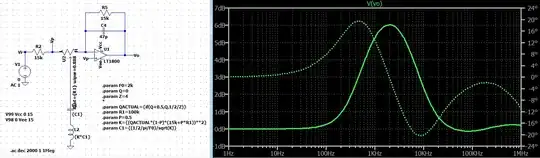
Here's the run for \$p=0.112\$:

Note that the bottom of the dip is right at \$2\:\text{kHz}\$ and \$-6\:\text{dB}\$. Just as predicted.
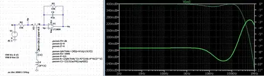
Here's the run for \$p=0.888\$:
Note that the top of the dip is right at \$2\:\text{kHz}\$ and \$+6\:\text{dB}\$. Also just as predicted.
Just FYI, though? \$C_1=19.59\:\text{nF}\$ and \$L_2=323.3\:\text{mH}\$. Those were computed from the chosen critical frequency and desired damping factor (when the potentiometer is right at midpoint position and given your resistor values, of course.)
(Also, the various non-idealities you see in the curves from about \$100\:\text{kHz}\$ and beyond come largely from \$C_4\$. If I set it close to zero then they go away and the curves look much closer to ideal curves.)


