What is a mesh, and why not instead use independent loops for mesh analysis?

Question

In the textbook "Fundamentals of Electric Circuits" by Alexander and Sadiku, 7th edition, p. 92, the definition of meshes depends on the the physical position of nodes. This doesn't make sense to me, because where you exactly you place your nodes should be irrelevant to the properties of the circuit.

The textbook attempts to define meshes using an example. It suggests that abcdefa is not a mesh, my understanding being the implication that there is another possible mesh, abefa, "interior" to it.

A mesh is a loop that does not contain any other loops within it. Fig. 3.17 (below), for example, paths abefa and bcdeb are meshes, but path abcdefa is not a mesh.

However, you can just tug the nodes around (in a way that clearly does not alter the circuit) so that for abefa and abcdefa, one is not "interior" to the other.

Is there a definition for mesh that is independent of how nodes are arranged, or can we just do away with the notion of meshes altogether and instead talk about a set of independent loops for "mesh" analysis?

Answer 1

Some of what I'll discuss is drawn from GRAPH THEORY AND ITS ENGINEERING APPLICATIONS by Wai-Kai Chen then at the University of Illinois, Chicago, and published in the Advanced Series in Electrical and Computer Engineering - Vol. 5, 1997, World Scientific Publishing Co. Pte. Ltd. Some will be drawn from several different books by Dr. Gilbert Strang.

Let's start with this directed graph example from Chapter 2 of Dr. Chen's paper, first, just to get across a basic idea:

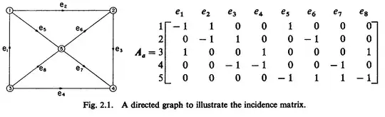
Now, I usually set up the directed graph matrix as the transpose of the incidence matrix shown above. But it's easy to do it either way and just recognize the meaning is the same so long as you keep track of which form you are working with. The results are the same, so long as you keep your mind straight.

I'm going to stop copying from the text of others and just draw things out in my own way. But I wanted to point out that mathematicians have been doing this stuff for quite some time.

Let's look at three directed graphs and see what the math tells us about them:

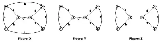
Let's use sympy/Python to define the incidence matrices as Dr. Chen shows us above:

# Incidence matrix for X:
X=Matrix([ [-1, 0, 1, 0, 0, 0, 0, 1, 0],
           [ 1, 1, 0, 0, 0, 0, 0, 0,-1],
           [ 0,-1,-1, 0, 0, 0, 1, 0, 0],
           [ 0, 0, 0, 1, 1, 0,-1, 0, 0],
           [ 0, 0, 0,-1, 0, 1, 0,-1, 0],
           [ 0, 0, 0, 0,-1,-1, 0, 0, 1] ])
Incidence matrix for Y:
Y=Matrix([ [-1, 0, 1, 0, 0, 0, 0],
           [ 1, 1, 0, 0, 0, 0, 0],
           [ 0,-1,-1, 0, 0, 0, 1],
           [ 0, 0, 0, 1, 1, 0,-1],
           [ 0, 0, 0,-1, 0, 1, 0],
           [ 0, 0, 0, 0,-1,-1, 0] ])
Incidence matrix for Z:
Z=Matrix([ [-1, 0, 1, 0, 0, 0],
           [ 1, 1, 0, 0, 0, 0],
           [ 0,-1,-1, 0, 0, 0],
           [ 0, 0, 0, 1, 1, 0],
           [ 0, 0, 0,-1, 0, 1],
           [ 0, 0, 0, 0,-1,-1] ])

(Note that all I did was remove the last two columns from X to get Y and then just the last column of Y to get Z. That removes the appropriate edges.)

Here, I stayed consistent with Dr. Chen's approach. I usually write these out as the transpose of the above, though. In any case, we can see the connectivity of the above in the following way:

# Connected nodes for X:
[[i for i in v] for v in X.transpose().nullspace()]
[[1, 1, 1, 1, 1, 1]]
Connected nodes for Y:
[[i for i in v] for v in Y.transpose().nullspace()]
[[1, 1, 1, 1, 1, 1]]
Connected nodes for Z:
[[i for i in v] for v in Z.transpose().nullspace()]
[[1, 1, 1, 0, 0, 0], [0, 0, 0, 1, 1, 1]]

This tells us quickly that figures X and Y are connected graphs but that Z is actually composed of two independent connected graphs. It works like this because the nullspace is \$\left\{v\mid A^T v=0\right\}\$. Put in other words its the set of vectors that must sum the directed arrows to zero. That's only guaranteed in X and Y if you include all the nodes into a single vector. But for Z that can be guaranteed for two distinct cases: one involving nodes 0, 1, and 2 and the other one involving nodes 3, 4, and 5 (looking at the rightmost diagram, of course.)

From this information you can immediately tell if you are working with one schematic, or more than one. (The transpose of the incidence matrix represents KCL.)

Let's now look at this another way:

# Meshes for X:
[[i for i in v] for v in X.nullspace()]
[[1, -1, 1, 0, 0, 0, 0, 0, 0],
 [0, 0, 0, 1, -1, 1, 0, 0, 0],
 [1, -1, 0, -1, 0, 0, -1, 1, 0],
 [0, 1, 0, 0, 1, 0, 1, 0, 1]]
Meshes for Y:
[[i for i in v] for v in Y.nullspace()]
[[1, -1, 1, 0, 0, 0, 0], [0, 0, 0, 1, -1, 1, 0]]
Meshes for Z:
[[i for i in v] for v in Z.nullspace()]
[[1, -1, 1, 0, 0, 0], [0, 0, 0, 1, -1, 1]]

This shows the meshes. The incidence matrix itself represents Ohm's law (KVL) and the nullspace represents all vectors along which the mapping collapses towards the origin (0.) In short, where the sum of the voltages as you move around a loop (KVL fashion) must go to zero. Which, of course, is just your meshes.

I'll get to X in a moment. But notice that there are the same two meshes each for Y and Z. Y, of course, as a single path between the meshes. But edge g cannot be part of a mesh in Y. (Not unless we add another edge with either a current source or a voltage source that connects the two meshes shown.)

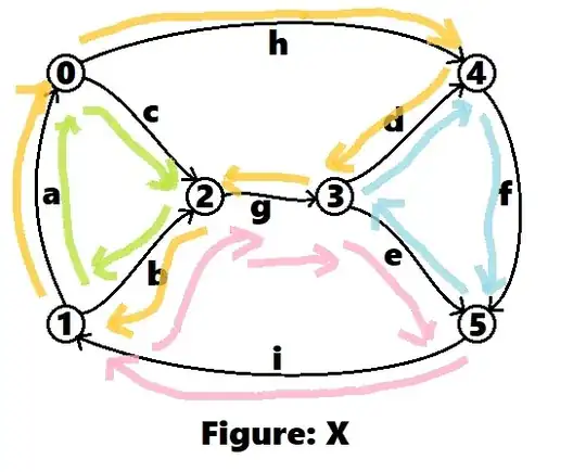
Note that we have four meshes given for X. \$\left[1, -1, 1, 0, 0, 0, 0, 0, 0\right]\$ says that if you take a loop that follows the edge a and c in their stated direction (positive means with the arrow) and edge b opposite its stated direction (negative means against the arrow) then you will have moved around a KVL loop that must sum to zero. The same is true for \$\left[0, 0, 0, 1, -1, 1, 0, 0, 0\right]\$, which is with d and f and against e. Then for \$\left[1, -1, 0, -1, 0, 0, -1, 1, 0\right]\$, which is with a and h and against b, d, and g. Then for \$\left[0, 1, 0, 0, 1, 0, 1, 0, 1\right]\$, which is with b, e, g and i.

I've colored in the meshes it found for X, below:

But you can always add or subtract these vectors to get a different vector. Suppose we didn't like these choices, but especially wanted one that covered the loop using edges a, h, f, and i. Then sum the appropriate loops:

#  Adding the orange, blue, and pink vectors:
[i for i in X.nullspace()[1]+X.nullspace()[2]+X.nullspace()[3]]
[1, 0, 0, 0, 0, 1, 0, 1, 1]

And there you go! The loop you wanted to get is there. Of course, this now combines information found in those three other loops, so just pick one of those to remove from the list of loops.

To see how that sum works so well, just notice that we start with the orange loop and add the blue one. The blue one has opposite values for edge d so d cancels out with the addition of the those two loops, adding e and f to make a new loop. But that's not enough. So adding the pink loop causes edges b, e and g to now be cancelled, while adding in edge i. That's how the desired loop was made.

All this gets into spanning spaces with vectors, matrix transformations generally, and the idea of rank as well as the Rank-Nullity Theorem (which has something important to say about how we must better understand the nullspaces.) Also note that the rank of the columnspace will always equal the rank of the rowspace, with the left and right nullspaces picking up the dimensional difference.

I'll leave the rest for now. You may review and ask questions.

(Added note: Just found this 1990 submission by Michael Parker in partial fulfillment for a masters degree at MIT and signed off by his Thesis advisor, Dr. Strang. It's worth reading and is accessible at no cost.)

Answer 2

You are absolutely correct about being able to shuffle nodes around to reveal alternative "meshes", and doing so does not alter the solution. The resulting equations will appear different, with terms in different places and equations, but those equations still embody the same information, and are describing the same system.

Furthermore, while that definition of mesh may exclude \$abcdef\$, using that loop will also produce the correct result. You can apply mesh analysis using the two loops shown below, as long as you are careful regarding current superposition:

^{simulate this circuit – Schematic created using CircuitLab}

For the orange loop, this would yield:

$$ \begin{aligned} V_1 - \overbrace{(I_1+I_2)}^{\text{add!}}R_1 - I_2R_3 &= 0 \\ \\ V_1 - I_1R_1 - I_2(R_1+R_3) &= 0 \\ \\ \end{aligned} $$

For the green loop:

$$ \begin{aligned} V_1 - (I_1+I_2)R_1 - I_1R_2 - V_2 &= 0 \\ \\ V_1 - V_2 - I_1(R_1 + R_2) - I_2R_1 &= 0 \\ \\ \end{aligned} $$

Solving this will yield exactly the same results as any simultaneous equations you get from applying mesh analysis for the two loops in the original schematic. From that perspective, the green loop above, \$abcdef\$, might also be considered a "mesh".

However, considering that the KVL equation for that green loop contains more terms (one per element) than you would find in the KVL equation for the right hand loop, this would probably involve more manipulation for the solution. It would make sense to keep things as simple as possible (the whole point of mesh analysis) and use the right hand loop instead of the green one.

In this sense, I think the definition of "mesh" as being "a loop that does not contain any other loops within it" is one of convenience, an optimisation to reduce the complexity of the simultaneous equations.