In my example, the transfer function is determined using the generalized form which shields you from applying a null-double injection or NDI. The principle is to reuse all the time constants already determined for the denominator and express high-frequency gains in which the energy-storing elements are alternatively set into their high-frequency states: a short circuit for a capacitor and an open circuit for an inductor. Then, combining these terms all together leads you to the numerator expression.
Now, to determine a resistance (or an impedance), the theoretical approach is to excite the port with a current source \$I_T\$ and express the voltage \$V_T\$ collected across its terminals:
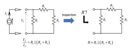
This method always work and can lead to complicated results, especially with controlled sources but, sometimes, you don't have choice. One alternative, is to consider inspecting the circuit: rather than applying a test generator, you "look" through the connecting terminals and infer, in your mind, the equivalent resistance you "see" or would measure with an ohm-meter. You can also do this inspection exercise by breaking down the circuit into a succession of simplified sketches of course.
The exercise is similar to find the high-frequency gains and the example you gave in the page you pasted is that of a transimpedance circuit shown below:
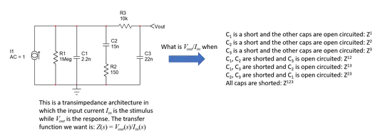
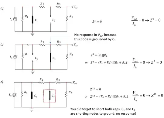
Here, you have to find the high-frequency transfer function linking the output voltage to the output current when the caps are alternatively shorted or open circuited. You immediately can see that if \$C_1\$ or \$C_3\$ are shorted, there is no response implying that the transfer function in these modes is zero. The only mode in which a response exists is when \$C_2\$ is shorted. In that case, the output voltage is simply \$V_{out}=I_{in}(R_1||R_2)\$ and thus \$\frac{V_{out}}{I_{in}}=Z^2=R_1||R_2\$. In this notation, the 2 in the exponent-like notation indicates that element 2 (\$C_2\$) is set in high frequency while the other are in dc state. In this configuration, \$R_3\$ does not participate because there is no current flowing into it. Should a resistance load \$V_{out}\$ in a different circuit, then, yes, \$R_3\$ would enter the picture but not here.
Now, if I look your sketch which is not the one I used in my example, this is a second-order circuit with \$C_1\$ and \$C_2\$ alternatively set in their high-frequency state or open circuited. When calculating the high-frequency gains, you forgot to short some of the caps. and there is no zero at all in this new circuit:
Now some comments triggered by your questions:
to determine the time constants of the denominator \$D(s)\$, the original stimulus is not used in the exercise. For instance, if you want to determine \$\frac{V_{out}}{V_{in}}\$, \$V_{in}\$ which is the stimulus applied to the input of your network is turned off and replaced by a 0-V source or a short circuit. Then, you apply the test generator method \$V_T\$ and \$I_T\$ (or inspection) to each of the energy-storing elements alternatively set in their dc or high-frequency state.
for the numerator \$N(s)\$, you can either apply a NDI but it can be intimidating to new comers or use the generalized form. This form builds on the already-determined time constants in \$D(s)\$ and you have to bring the stimulus back. Then, you determine the gains of your circuit - \$\frac{V_{out}}{V_{in}}\$ for instance - when the energy-storing elements are alternatively set in dc or high-frequency state. It is usually simple as any cap. shorting the path to the output immediately brings 0 in the transfer function. If not, like with \$R_1\$ in my figure, then it indicates that there is a zero in the transfer function.
Based on the suggested responses you gave in your drawing, it looks like you were calculating impedances while \$I_{in}\$ was brought back. If \$I_{in}\$ is there, then you have to consider the high-frequency gains only. Let me know if it makes better sense now and congrats for learning the FACTs, this is one the best tools to acquire!


