Linear algebra (Osnabrück 2024-2025)/Part II/Lecture 54

Stochastic matrices

Definition

A real square matrix

{}M={\left(a_{ij}\right)}_{1\leq i,j\leq n}\,

is called column stochastic matrix if all entries

{}a_{ij}\geq 0\,,

and every column sum (that is, for every ${}j$ ), is

{}\sum _{i=1}^{n}a_{ij}=1\,.

The basic interpretation for a column stochastic matrix is the following: There is a set of ${}n$ possible places, spots, positions, vertices in a network, web pages, etc., where someone or something can be with a certain probability (a distribution, a weighting). Such a distribution is described by an ${}n$ -tuple ${}{\begin{pmatrix}v_{1}\\v_{2}\\\vdots \\v_{n}\end{pmatrix}}$ with real non-negative numbers ${}v_{i}$ satisfying ${}\sum _{i=1}^{n}v_{i}=1$ . This is also called a distribution vector. A column stochastic matrix describes the transition probability in the given network in a certain time segment. The entry ${}a_{ij}$ is the probability that an object being at the vertex ${}j$ (a visitor of the web page ${}j$ ) moves to the position ${}i$ (goes to the webpage ${}i$ ). The ${}j$ -th standard vector corresponds to the distribution where everything is in the vertex ${}j$ .The ${}j$ -th column of the matrix describes the image of this standard vector under the matrix. In general, for a given distribution ${}v$ , applying the matrix computes the image distribution ${}Mv$ ; see Exercise 54.1 . A natural question is whether there are distributions that are stationary (stationary distribution, or fixed distribution, or eigendistribution), that is, they are transformed to themselves, or whether there exist periodic distributions, or whether there exist limit distributions, and how to compute them.

Example

A column stochastic ${}2\times 2$ -matrix has the form

{\begin{pmatrix}p_{1}&p_{2}\\1-p_{1}&1-p_{2}\end{pmatrix}}

wit

{}0\leq p_{1},p_{2}\leq 1\,.

The characteristic polynomial is

{}{\begin{aligned}(X-p_{1})(X-1+p_{2})-(1-p_{1})p_{2}&=X^{2}+(p_{2}-p_{1}-1)X+p_{1}(1-p_{2})-p_{2}(1-p_{1})\\&=X^{2}+(p_{2}-p_{1}-1)X+p_{1}-p_{2}\\&=(X-1)(X+p_{2}-p_{1}).\,\end{aligned}}

Eigenvalues are ${}1$ and ${}p_{1}-p_{2}$ . A stationary distribution is (exclude the cases ${}p_{1}=1$ and ${}p_{2}=0$ for the following computation) given by ${}{\begin{pmatrix}{\frac {p_{2}}{p_{2}-p_{1}+1}}\\{\frac {1-p_{1}}{p_{2}-p_{1}+1}}\end{pmatrix}}$ , because of

{}{\begin{aligned}{\begin{pmatrix}p_{1}&p_{2}\\1-p_{1}&1-p_{2}\end{pmatrix}}{\begin{pmatrix}{\frac {p_{2}}{p_{2}-p_{1}+1}}\\{\frac {1-p_{1}}{p_{2}-p_{1}+1}}\end{pmatrix}}&={\begin{pmatrix}p_{1}{\frac {p_{2}}{p_{2}-p_{1}+1}}+p_{2}{\frac {1-p_{1}}{p_{2}-p_{1}+1}}\\(1-p_{1}){\frac {p_{2}}{p_{2}-p_{1}+1}}+(1-p_{2}){\frac {1-p_{1}}{p_{2}-p_{1}+1}}\end{pmatrix}}\\&={\begin{pmatrix}{\frac {p_{1}p_{2}+p_{2}(1-p_{1})}{p_{2}-p_{1}+1}}\\{\frac {(1-p_{1})p_{2}+(1-p_{2})(1-p_{1})}{p_{2}-p_{1}+1}}\end{pmatrix}}\\&={\begin{pmatrix}{\frac {p_{2}}{p_{2}-p_{1}+1}}\\{\frac {1-p_{1}}{p_{2}-p_{1}+1}}\end{pmatrix}}.\end{aligned}}

Example

The column stochastic ${}2\times 2$ -matrix

{\begin{pmatrix}0&1\\1&0\end{pmatrix}}

transforms the distribution ${}{\begin{pmatrix}p\\1-p\end{pmatrix}}$ into the distribution ${}{\begin{pmatrix}1-p\\p\end{pmatrix}}$ . The contribution ${}{\begin{pmatrix}{\frac {1}{2}}\\{\frac {1}{2}}\end{pmatrix}}$ is transformed to itself, that is, it is a stationary distribution. The distribution ${}{\begin{pmatrix}1\\0\end{pmatrix}}$ is transformed into ${}{\begin{pmatrix}0\\1\end{pmatrix}}$ , and vice versa. It is a periodic distribution, the period length is ${}2$ .

Example

The column stochastic ${}n\times n$ -matrix

{\begin{pmatrix}1&1&\cdots &1\\0&0&\cdots &0\\\vdots &\vdots &\ddots &\vdots \\0&0&\cdots &0\end{pmatrix}}

transforms the distribution ${}{\begin{pmatrix}v_{1}\\\vdots \\v_{n}\end{pmatrix}}$ into the distribution

{}{\begin{pmatrix}1&1&\cdots &1\\0&0&\cdots &0\\\vdots &\vdots &\ddots &\vdots \\0&0&\cdots &0\end{pmatrix}}{\begin{pmatrix}v_{1}\\v_{2}\\\vdots \\v_{n}\end{pmatrix}}={\begin{pmatrix}\sum _{i=1}^{n}v_{i}\\0\\\vdots \\0\end{pmatrix}}={\begin{pmatrix}1\\0\\\vdots \\0\end{pmatrix}}\,.

The first standard vector is an eigenvector of the eigenvalue ${}1$ ; every other standard vector, and in fact every distribution vector, is transformed into the first standard vector. The kernel is generated by the vectors ${}e_{1}-e_{j}$ , ${}j\geq 2$ , and does not contain any distribution vector.

Example

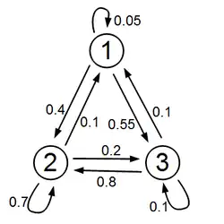
Let ${}N$ be a network (a "directed graph“), consisting in a set ${}K$ of vertices, and a set of directed edges, which can exist between the vertices. For example, ${}K$ is the set of all web pages, and there exists an arrow from ${}j\in K$ to ${}i\in K$ , if the web page ${}j$ has a link to the web page ${}i$ . The linking structure can be expressed by the adjacency matrix

{}A={\left(a_{ij}\right)}\,,

where

{}a_{ij}:={\begin{cases}1,\,{\text{there exists a link from }}j{\text{ to }}i,\\0,\,{\text{ else}},\end{cases}}\,,

or by the column stochastic matrix

{}B={\left(b_{ij}\right)}\,,

where

{}b_{ij}={\frac {a_{ij}}{d_{j}}}\,,

and ${}d_{j}$ is the number of links starting at the vertex ${}j$ . This division ensures that the column sum equals ${}1$ (we suppose that there is at least one link starting at any vertex).

The adjacency matrix, and the column stochastic version of the adjacency matrix of the graph on the right (where we add always self links) are

{\begin{pmatrix}1&0&0&0&0\\1&1&0&0&0\\1&0&1&0&0\\1&1&1&1&0\\1&0&1&1&1\end{pmatrix}}{\text{ and }}{\begin{pmatrix}{\frac {1}{5}}&0&0&0&0\\{\frac {1}{5}}&{\frac {1}{2}}&0&0&0\\{\frac {1}{5}}&0&{\frac {1}{3}}&0&0\\{\frac {1}{5}}&{\frac {1}{2}}&{\frac {1}{3}}&{\frac {1}{2}}&0\\{\frac {1}{5}}&0&{\frac {1}{3}}&{\frac {1}{2}}&1\end{pmatrix}}.

Powers of a stochastic matrix

We investigate now the powers of a stochastic matrix with the help of the sum norm and the results of the last lecture.

Corollary

A column stochastic matrix is

stable.

Proof

For an arbitrary vector ${}v\in V$ , we have

{}{\begin{aligned}\mid \mid \!Mv\!\mid \mid _{\operatorname {sum} }&=\sum _{i=1}^{n}\vert {(Mv)_{i}}\vert \\&=\sum _{i=1}^{n}\vert {\sum _{j=1}^{n}a_{ij}v_{j}}\vert \\&\leq \sum _{i=1}^{n}{\left(\sum _{j=1}^{n}a_{ij}\vert {v_{j}}\vert \right)}\\&=\sum _{j=1}^{n}\vert {v_{j}}\vert {\left(\sum _{i=1}^{n}a_{ij}\right)}\\&=\sum _{j=1}^{n}\vert {v_{j}}\vert \\&=\mid \mid \!v\!\mid \mid _{\operatorname {sum} }.\end{aligned}}

Iterative application of this observation shows that Theorem 53.10 (2) is satisfied.

\Box

Lemma

Let

{}M={\left(a_{ij}\right)}_{1\leq i,j\leq n}\,

be a real square matrix with non-negative entries. Then ${}M$ is column stochastic if and only if ${}M$ is isometric with respect to the sum norm for vectors with non-negative entries, that is,

{}\Vert {Mv}\Vert _{\rm {sum}}=\Vert {v}\Vert _{\rm {sum}}\,

holds for all

{}v\in \mathbb {R} _{\geq 0}^{n}

.

Proof

Let ${}M$ be a column stochastic matrix, and

{}v={\begin{pmatrix}v_{1}\\\vdots \\v_{n}\end{pmatrix}}\,

be a vector with non-negative entries. Then

{}{\begin{aligned}\Vert {Mv}\Vert _{\rm {sum}}&=\sum _{i=1}^{n}(Mv)_{i}\\&=\sum _{i=1}^{n}{\left(\sum _{j=1}^{n}a_{ij}v_{j}\right)}\\&=\sum _{j=1}^{n}v_{j}{\left(\sum _{i=1}^{n}a_{ij}\right)}\\&=\sum _{j=1}^{n}v_{j}\\&=\Vert {v}\Vert _{\rm {sum}}\end{aligned}}

holds. If the described isometric property holds, then it holds in particular for the images of the standard vectors. That means that their sum norm equals ${}1$ . These images are the corresponding columns of the matrix; therefore, all column sums are ${}1$ .

\Box

Lemma

Let ${}M$ be a

column stochastic matrix. Then the following statements hold.

There exists eigenvectors to the eigenvalue ${}1$ .
If there exists a row such that all its entries are positive, then for every vector ${}v\in V$ that has a positive and also a negative entry, the estimate
${}\mid \mid \!Mv\!\mid \mid _{\operatorname {sum} }<\mid \mid \!v\!\mid \mid _{\operatorname {sum} }\,$

holds.
If there exists a row such that all its entries are positive, then the eigenspace of the eigenvalue ${}1$ is one-dimensional. There exists an eigenvector where all entries are no-negative; in particular, there is a uniquely determined stationary distribution.

Proof

The transposed matrix is row stochastic; therefore, it has an eigenvector ${}{\begin{pmatrix}1\\1\\\vdots \\1\end{pmatrix}}$ to the eigenvalue ${}1$ . Due to Theorem 23.2 , the characteristic polynomial of the transposed matrix has a zero at ${}1$ . Because of Exercise 23.19 , this also holds for the matrix we have started with. Hence, ${}M$ has an eigenvector to the eigenvalue ${}1$ .
We now assume also that all entries of the ${}k$ -th row are positive, and let ${}v\in V$ denote a vector with (at least) a positive and a negative entry. Then
${}{\begin{aligned}\mid \mid \!Mv\!\mid \mid _{\operatorname {sum} }&=\sum _{i=1}^{n}\vert {(Mv)_{i}}\vert \\&=\sum _{i=1}^{n}\vert {\sum _{j=1}^{n}a_{ij}v_{j}}\vert \\&=\sum _{i\neq k}\vert {\sum _{j=1}^{n}a_{ij}v_{j}}\vert +\vert {\sum _{j=1}^{n}a_{kj}v_{j}}\vert \\&<\sum _{i\neq k}\sum _{j=1}^{n}a_{ij}\vert {v_{j}}\vert +\sum _{j=1}^{n}\vert {a_{kj}v_{j}}\vert \\&=\sum _{i=1}^{n}\sum _{j=1}^{n}a_{ij}\vert {v_{j}}\vert \\&=\sum _{j=1}^{n}\vert {v_{j}}\vert {\left(\sum _{i=1}^{n}a_{ij}\right)}\\&=\sum _{j=1}^{n}\vert {v_{j}}\vert \\&=\mid \mid \!v\!\mid \mid _{\operatorname {sum} }\end{aligned}}$

holds.
As in the proof of (2), let all entries of the ${}k$ -th row be positive. For any eigenvector ${}v$ to the eigenvalue ${}1$ , according to (2), either all entries are non-negative, or non-positive. Hence, for such a vector, because of ${}Mv=v$ , its ${}k$ -th entry is not ${}0$ . Let ${}v,w$ be such eigenvectors. Then ${}{\frac {w_{k}}{v_{k}}}v-w$ belongs to the fixed space. However, the ${}k$ -th component of this vector equals ${}0$ ; therefore, it is the zero vector. This means that ${}v$ and ${}w$ are linearly dependent. Therefore, this eigenspace is one-dimensional. Because of (2), there exists an eigenvector to the eigenvalue ${}1$ with non-negative entries. By normalizing, we get a stationary distribution.

\Box

Example

We consider the column stochastic ${}3\times 3$ -matrix

{\begin{pmatrix}{\frac {1}{3}}&{\frac {1}{3}}&{\frac {1}{3}}\\{\frac {1}{2}}&{\frac {2}{3}}&0\\{\frac {1}{6}}&0&{\frac {2}{3}}\end{pmatrix}};

here, all entries of the first row are positive. Due to Lemma 54.8 , there exists a unique eigendistribution. In order to determine this distribution, we compute the kernel of

{}{\begin{pmatrix}1&0&0\\0&1&0\\0&0&1\end{pmatrix}}-{\begin{pmatrix}{\frac {1}{3}}&{\frac {1}{3}}&{\frac {1}{3}}\\{\frac {1}{2}}&{\frac {2}{3}}&0\\{\frac {1}{6}}&0&{\frac {2}{3}}\end{pmatrix}}={\begin{pmatrix}{\frac {2}{3}}&-{\frac {1}{3}}&-{\frac {1}{3}}\\-{\frac {1}{2}}&{\frac {1}{3}}&0\\-{\frac {1}{6}}&0&{\frac {1}{3}}\end{pmatrix}}\,.

This kernel is generated by ${}{\begin{pmatrix}2\\3\\1\end{pmatrix}}$ , and the stationary distribution is

{}{\begin{pmatrix}{\frac {2}{6}}\\{\frac {3}{6}}\\{\frac {1}{6}}\end{pmatrix}}={\begin{pmatrix}{\frac {1}{3}}\\{\frac {1}{2}}\\{\frac {1}{6}}\end{pmatrix}}\,.

Example

For the column stochastic ${}3\times 3$ -matrix

{\begin{pmatrix}1&0&{\frac {1}{3}}\\0&1&{\frac {1}{3}}\\0&0&{\frac {1}{3}}\end{pmatrix}},

the eigenspace to the eigenvalue ${}1$ equals ${}\langle e_{1},\,e_{2}\rangle$ ;, it is two-dimensional. This shows that the conclusion of Lemma 54.8 does not hold even when there exists a column (but not a row) with strictly positive entries.

Theorem

Let ${}M$ be a column stochastic matrix, fulfilling the property that there exists a row in which all entries are positive. Then for every distribution vector ${}v\in \mathbb {R} _{\geq 0}^{n}$ with ${}\sum _{i=1}^{n}v_{i}=1$ , the sequence ${}M^{n}v$ converges to the uniquely determined stationary distribution

of

{}M

.

Proof

Let ${}w\in \mathbb {R} ^{n}$ be the stationary distribution, which is uniquely determined because of Lemma 54.8 (3). We set

{}U={\left\{{\begin{pmatrix}u_{1}\\\vdots \\u_{n}\end{pmatrix}}\mid \sum _{i=1}^{n}u_{i}=0\right\}}\subseteq \mathbb {R} ^{n}\,.

This is a linear subspace of ${}\mathbb {R} ^{n}$ of dimension ${}n-1$ . Due to Lemma 54.8 (2), ${}w$ has only non-negative entries; therefore, it does not belong to ${}U$ . Because of

{}{\begin{aligned}\sum _{i=1}^{n}(Mu)_{i}&=\sum _{i=1}^{n}{\left(\sum _{j=1}^{n}a_{ij}u_{j}\right)}\\&=\sum _{j=1}^{n}u_{j}{\left(\sum _{i=1}^{n}a_{ij}\right)}\\&=\sum _{j=1}^{n}u_{j},\end{aligned}}

${}U$ is invariant under the matrix ${}M$ . Hence,

{}V=U\oplus \mathbb {R} w\,

is a direct sum decomposition into invariant linear subspaces. For every ${}u\in U$ with ${}\mid \mid \!u\!\mid \mid _{\operatorname {sum} }=1$ , we have

{}\mid \mid \!Mu\!\mid \mid _{\operatorname {sum} }<1\,

due to Lemma 54.8 (2). The sphere of radius ${}1$ is compact with respect to every norm; therefore, the induced maximum norm of ${}M{|}_{U}$ is smaller than ${}1$ . Because of Lemma 53.8 and Theorem 53.6 , the sequence ${}M^{n}u$ converges for every ${}u\in U$ to the zero vector.

Let now ${}v\in V$ be a distribution vector; because of

{}\sum _{i=1}^{n}v_{i}=1=\sum _{i=1}^{n}w_{i}\,,

we can write

{}v=w+u\,

with ${}u\in U$ . Because of

{}M^{n}v=M^{n}(w+u)=M^{n}w+M^{n}u=w+M^{n}u\,,

and the reasoning before, this sequence converges to ${}w$ .

\Box

Remark

In the situation of Lemma 54.8 , we can find the eigendistribution by solving a system of linear equations. If we are dealing with a huge matrix (think about ${}\geq 10^{9}$ vertices), then such a computation time-consuming. Often, it is not necessary to know the eigendistribution precisely; it is enough to know a good approximation. For this, we may start with an arbitrary distribution, and we compute finitely many iterations. Because of Theorem 54.11 , we know that this method gives arbitrarily good approximations of the eigendistribution. For example, a search engine for the web generates for search item an ordered list of web pages where this search item occurs. How does this ordering arise? The true answer is, at least for the first entries, that it depends on how much someone has paid. Despite of this, it is a natural approach, and this is also the basis for the Page ranks, to consider the numerical ordering in the eigendistribution. The first entry is the one where most people would "finally“ end up when they follow with the same probability any possible link. This movement is modelled^[1] by the stochastic matrix described in Example 54.5 .

The numerical difference between finding an exact solution of a system of linear equations to determine an eigenvector, and the power method, can be grasped in the following way. Let an ${}n\times n$ -matrix be given. The elimination process needs in order to eliminate the first variable in ${}n-1$ equations, ${}n(n-1)\sim n^{2}$ multiplications (here, we do not consider the easier additions); therefore, the seize of the multiplications in the complete elimination process is

{}n^{2}+(n-1)^{2}+(n-2)^{2}+\cdots +1\sim {\frac {1}{6}}n^{3}\,.

For the evaluation of the matrix at a vector, ${}n^{2}$ multiplications are necessary. If we want to compute ${}k$ iterations, we need ${}kn^{2}$ operations. Hence, if ${}k$ is substantially smaller than ${}n$ , then thetotal expenditure is substantially smaller.

Footnotes

↑
Modelling means in (in particular, applied) mathematics the process to understand phenomena of the real world with mathematical tools. We model physical processes, weather phenomena, transactions in finance, etc.

<< \| Linear algebra (Osnabrück 2024-2025)/Part II \| >> PDF-version of this lecture Exercise sheet for this lecture (PDF)

[1] 
Modelling means in (in particular, applied) mathematics the process to understand phenomena of the real world with mathematical tools. We model physical processes, weather phenomena, transactions in finance, etc.

[1]