I'm using Qutip to plot some basic two level dynamics using hamiltonians with a temporal envelope defined as the sum of two error functions, designed to make it more representative of experimental conditions.
I'm using the following code.
import numpy as np
from qutip import *
from scipy.special import erf
import matplotlib.pyplot as plt

def pulseEdge(x, x0, sigma):
    pulseEdge = ((erf((x-x0)/sigma)) +1.)/2.
    return pulseEdge

def pulse(t, tOn, tOff, sigma):
    return pulseEdge(t, tOn, sigma)* (1.-pulseEdge(t, tOff, sigma))

def H(t, args):
    H = Qobj([[0.,1],[1,0.0]])
    envelope = pulse(t, 2,2+np.pi/2,0.2)
    return H*envelope

tlist = np.linspace(0,10,1000)
h = np.array([H(t,0)[0][0] for t in tlist])
H_list = H

psi0 = basis(2,0)
basisStates = [basis(2,i) for i in range(2)]
e_ops = [b*b.dag() for b in basisStates]

me =mesolve(H_list, psi0, tlist,  progress_bar = None, e_ops = e_ops)

plt.plot(me.expect[0])
plt.plot(me.expect[1])

plt.plot(h)
plt.show()
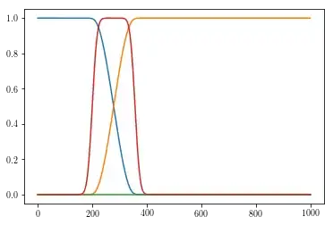
Which works really well and produces the desired output, a $\pi$ Rabi oscillation driven by a $\pi$ pulse. The red is the envelope of the Rabi hamiltonian, and the orange and blue are the (expected) populations of the upper and lower states of a two level system undergoing a pi pulse. This is the expected behaviour.
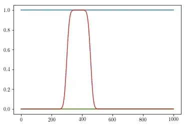
Except if I want the pulse one time unit later, when no evolution is driven. The code is exactly the same, except the hamiltonian function is modified to the following
def H(t, args):
    H = Qobj([[0.,1],[1,0.0]])
    envelope = pulse(t, 3,3+np.pi/2,0.2)
    H*=envelope
    return H
which produces
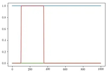
Or if I want the edges to be sharper, when again, no evolution occurs
def H(t, args):
    H = Qobj([[0.,1],[1,0.0]])
    envelope = pulse(t, 2,2+np.pi/2,0.01)
    H*=envelope
    return H
What element of these time dependent Hamiltonians functions is causing mesolve to correctly calculate the dynamics in some cases, and completely fail in others?
The difference between the Hamiltonians in the above plots seems minor and arbitrary to me, and the rest of the code is identical between plots.
EDIT
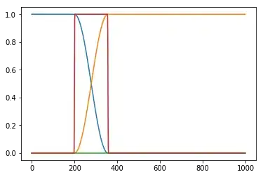
After Paul Nation's answer, here is updated, working code.
import numpy as np
from qutip import *
from scipy.special import erf
import matplotlib.pyplot as plt

def pulseEdge(x, x0, sigma):
    pulseEdge = ((erf((x-x0)/sigma)) +1.)/2.
    return pulseEdge

def pulse(t, tOn, tOff, sigma):
    return pulseEdge(t, tOn, sigma)* (1.-pulseEdge(t, tOff, sigma))

def H(t, args):
    H = Qobj([[0.,1],[1,0.0]])
    envelope = pulse(t, 2,2+np.pi/2,0.01)
    H*=envelope
    return H

tlist = np.linspace(0,10,1000)
h = np.array([H(t,0)[0][0] for t in tlist])
H_list = H

psi0 = basis(2,0)
basisStates = [basis(2,i) for i in range(2)]
e_ops = [b*b.dag() for b in basisStates]

options = Options(max_step = 1)
me =mesolve(H_list, psi0, tlist,  progress_bar = None, e_ops = e_ops, options = options)

plt.plot(me.expect[0])
plt.plot(me.expect[1])

plt.plot(h)
plt.show()


