The required fidelity $F$ is a function of the Cartesian product of the single $n$-qubit state space: $CP^{2^n-1}$ and $n$ copies of a single qubit state space: $CP^{1} \cong S^2$. The statistics of $F$ is computed for a sample space drawn uniformly from the state space regarded as a probability space with respect to its Fubini-Study measure.
An explicit expression of $F$ is given in coordinates, and the assumption of the average: $<F> = \frac{1}{2^n}$ is validated by a direct integration.
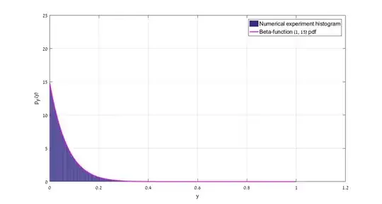
Next, the probability density function of $F$ is computed again by a direct integration (and found to be a beta distribution with parameters $\alpha = 1$, $\beta = 2^n-1$).
The computation results are compared to a numerical experiment with $n=4$.
Finally, the required probability is explicitly computed from the density function.
We can parametrize the complex projective space $CP^{N-1}$, almost everywhere with the coordinates $ \mathbb{C}^{N-1} \ni \mathbf{\zeta} = \{[\zeta_1, . . ., \zeta_{N-1}]^t\}$. A random $N$-dimensional normalized vector corresponding to the point $\mathbf{\zeta}$ is given by (as a column vector):
$$|\psi(\mathbf{\zeta}, \mathbf{\bar{\zeta}})\rangle = \frac{[1, \zeta _1,.,.,., \zeta _{N-1}]^t}{\sqrt{1+\mathbf{\zeta}^{\dagger} \mathbf{\zeta} }}$$
(We will eventually take $N=2^n$ or $N=2$). The Fubini-Study volume element is given by:
$$d{\mu}_{CP^{N-1}}(\mathbf{\zeta}, \mathbf{\bar{\zeta}}) = \frac{(N-1)!}{\pi^{N-1}}\frac{\prod_{k=1}^{N-1} d\zeta_k d\bar{\zeta}_k}{(1+\mathbf{\zeta}^{\dagger} \mathbf{\zeta})^N}$$
(The prefactor serves for normalizing the volume to a unit mass).
The following integral identities are valid:
$$\int_{CP^{N-1}} \frac{\zeta_k } {(1+\mathbf{\zeta}^{\dagger} \mathbf{\zeta})^N} d{\mu}_{CP^{N-1}}(\mathbf{\zeta}, \mathbf{\bar{\zeta})} = 0$$
$$\int_{CP^{N-1}} \frac{\bar{\zeta}_k } {(1+\mathbf{\zeta}^{\dagger} \mathbf{\zeta})^N} d{\mu}_{CP^{N-1}}(\mathbf{\zeta}, \mathbf{\bar{\zeta})} = 0$$
$$\int_{CP^{N-1}} \frac{1} {(1+\mathbf{\zeta}^{\dagger} \mathbf{\zeta})^N} d{\mu}_{CP^{N-1}}(\mathbf{\zeta}, \mathbf{\bar{\zeta})} = \frac{1}{N}$$
$$\int_{CP^{N-1}} \frac{\zeta_k\bar{\zeta}_l } {(1+\mathbf{\zeta}^{\dagger} \mathbf{\zeta})^N} d{\mu}_{CP^{N-1}}(\mathbf{\zeta}, \mathbf{\bar{\zeta})} = \frac{1}{N}\delta_{kl}$$
The Fubini-Study volume element is invariant with respect to the following unitary transformation realized non-linearly on the coordinates:
Let $U \in U(N)$ be given in the following block form:
$$U = \begin{bmatrix}
a & \mathbf{b}^t\\
\mathbf{c} & D
\end{bmatrix}$$
($a$ is a scalar, $b$ and $c$ are $N-1$ dimensional column vectors and $D$ is an $N-1\times N-1$ matrix).
$$\begin{bmatrix} 1\\ \mathbf{\zeta} \end{bmatrix} \rightarrow \begin{bmatrix} 1\\ \mathbf{\zeta}' \end{bmatrix} = (a + \mathbf{b}^t \zeta)\, U \begin{bmatrix} 1\\ \mathbf{\zeta} \end{bmatrix}$$
The first factor is a multiplier (cocycle).
Similarly, the $k$-th single qubit complex projective line can be parametrized almost everywhere by:
$$|\alpha_k(z_k, \bar{z}_k)\rangle = \frac{[1, z_k]^t}{\sqrt{1+\bar{z_k} z_k }}$$
And the corresponding volume element:
$$d{\mu}_{CP^{1}}(z_k, \bar{z}_k) = \frac{1}{\pi}\frac{dz_k d\bar{z_k}}{(1+\bar{z_k} z_k)^2}$$
Denoting by $f$ the natural mapping from the power set of $\mathbb{Z}_{n} = \{0, .,.,., n-1\}$ to $\mathbb{Z}_{2^n}$:
$$f(x) = \sum_{k \in x} 2^k$$
and using the shorthand notation:
$$z^{ f(x) } = \prod_{ k\in x } z_k$$
(with the convention $\zeta_0 = z_0 = 1$)
Tensoring the single qubit vectors and performing the inner product, we get:
$$F(\mathbf{\zeta}, z_0, ., ., . z_{n-1}, \mathbf{\bar{\zeta}}, \bar{z}_0, ., ., . \bar{z}_{n-1})= \frac{|\sum_{x \in \mathcal{P}(\mathbb{Z}_{n})} \zeta_{f(x)} \bar{z}^{f(x)} |^2}{(1+\mathbf{\zeta}^{\dagger} \mathbf{\zeta}) \prod_{k \in \mathbb{Z}_{n}} (1+\bar{z_k} z_k)}$$
The average of $F$ is computed by means of the following integral:
$$<F> = \int_{CP^{2^n-1}} d{\mu}_{CP^{N-1}}(\mathbf{\zeta}, \mathbf{\bar{\zeta}}) \prod_{k=0}^{N-1} d{\mu}_{CP^{1}}(z_k, \bar{z}_k) F(\mathbf{\zeta}, z_0, ., ., . z_{n-1}, \mathbf{\bar{\zeta}}, \bar{z}_0, ., ., . \bar{z}_{n-1})$$
Expanding the numerator of $F$, we get a quadratic polynomial in $\mathbf{\zeta}, \mathbf{\bar{\zeta}}$. Using the integration formulas, only $2^n$ terms survive, each contributing $\frac{1}{2^n}$. Thus, we are left with:
$$<F> = \frac{1}{2^n} \prod_{k=0}^{N-1} d{\mu}_{CP^{1}}(z_k, \bar{z}_k) \frac{\sum_{x \in \mathcal{P}(\mathbb{Z}_{n})} z^{f(x)} \bar{z}^{f(x)} }{ \prod_{k \in \mathbb{Z}_{n}} (1+\bar{z_k} z_k)}$$
The numerator factors to the denominator, and we are left with a product of $2^n$ normalized volumes of $CP^1$, i.e. $1$,
Thus
$$<F> = \frac{1}{2^n}$$
Given the explicit expression of the function $F$ on a probability space; its probability density function can be written as:
$$p_F(y) = \int_{CP^{2^n-1}} d{\mu}_{CP^{N-1}}(\mathbf{\zeta}, \mathbf{\bar{\zeta}}) \prod_{k=0}^{N-1} d{\mu}_{CP^{1}}(z_k, \bar{z}_k) \delta(F(\mathbf{\zeta}, z_0, ., ., . z_{n-1}, \mathbf{\bar{\zeta}}, \bar{z}_0, ., ., . \bar{z}_{n-1}) – y)$$
We observe that the numerator of $F$ can be written as:
$$\begin{bmatrix}1 & \bar{\mathbf{\zeta}}\end{bmatrix}
\begin{bmatrix}1 \\ \mathbf{z}\end{bmatrix}
\begin{bmatrix}1 & \bar{\mathbf{z}}\end{bmatrix}
\begin{bmatrix}1 \\ \mathbf{\zeta}\end{bmatrix}$$
The interior matrix (depending on $\mathbf{z}$ only) is of unit rank; thus it can be diagonalized by a unitary transformation to a matrix of the form:
$$ \mathrm{diag }\begin{bmatrix} 1+ \mathbf{z}^{\dagger} \mathbf{z}, & 0, & 0, & ... \end{bmatrix}$$
(Please notice that the scalar cocycles cancel between the numerator and the denominator and the Fubini-Study measure is invariant under the transformation).
As mentioned above, the nonvanishing first element just factors out to the denominator depending on $z$. Thus, we are left with $n$ integrations on the normalized volumes of $CP^1$ giving an overall result of $1$ with respect to the $z$ integration. As for the $\zeta$ dependent terms, we are left with only one term of $\begin{bmatrix}1 & \bar{\mathbf{\zeta}}\end{bmatrix} \begin{bmatrix}1 \\ \mathbf{\zeta}\end{bmatrix}$, which can be taken the first, i.e., $1$, thus the delta function term becomes:
$$\delta(\frac{1}{(1+\mathbf{\zeta}^{\dagger} \mathbf{\zeta})}-y)$$
Performing the standard manipulations on the delta function, we obtain:
$$\frac{1}{2y^{\frac{3}{2}}(1-y)^{\frac{1}{2}}}\delta(\sqrt{\mathbf{\zeta}^{\dagger} \mathbf{\zeta}}-\sqrt{\frac{1-y}{y}})$$
The constraint is a spherical surface of dimension $2N-3$ inside $CP^{N-1}$ and radius $\sqrt{\frac{1-y}{y}}$
Using the surface area formula for a $n-1$ sphere of unit radius:
$$S_{n-1} = \frac{n \pi^{\frac{n}{2}}}{\Gamma(\frac{n}{2}+1)}$$
We arrive at:
$$ p_F(y) = \frac{1}{2y^{\frac{3}{2}}(1-y)^{\frac{1}{2}}} \frac{(2N-2) \pi^{N-1}}{\Gamma(N)} \left(\sqrt{\frac{1-y}{y}}\right)^{2N-3} \frac{(N-1)!}{\pi^{N-1}} y^N = (N-1)(1-y)^{N-2}$$
Which is just the beta distribution, with the parameters $\alpha = 1$, $\beta = 2^n-1$).
Thus, for the $n$ qubit case, we have:
$$ p_F(y) = = (2^n-1)(1-y)^{2^n-2}$$
A numerical experiment was performed with $n=4$ with $10^6$ draws. The following figure compares the computed probability density function to the experiment's histogram:
From the probability density function, we get asymptotically for n>>1 and $\epsilon>>\frac{1}{2^n}$:
$$\mathrm{Pr}(y>\frac{1}{2^n}+\epsilon) = e^{-2^n\epsilon}$$
