If a state is only "close to" an eigenstate of an operator, how many applications of the operator does it take to scramble the state?

Question

Suppose we have an operator $U$, and a register $|\lambda\rangle$ in an eigenstate of $U$ with eigenvalue $\lambda=1$. Repeatedly applying $U$ to $|\lambda\rangle$ does not affect $|\lambda\rangle$ - that is, $\langle\lambda|U^r|\lambda\rangle=1$ for all $r\in \mathbb{Z}$.

However suppose we have another register $|\mu\rangle$, which is only "close to" the eigenstate $|\lambda\rangle$. That is, suppose we have a state $|\mu\rangle$ with $\langle\lambda|\mu\rangle=1-\delta$, for some small $\delta$. I believe repeated applications of $U$ will eventually scramble $|\mu\rangle$ beyond recognition. But, with respect to $\delta$, how quickly does this scrambling take place?

How much do we have to know about $U$ and $\langle\lambda|\mu\rangle$ to be able to say anything about how big $r$ has to be before $\langle\mu|U^r|\mu\rangle\lt 1/3$?

I think this is akin to asking for more spectral properties of $U$. Do we need to know about other eigenvalues of $U$ to answer how big $\delta$ has to be before $\langle\mu|U^r|\mu\rangle\lt 1/3$?

If we are able to prepare two separate registers, both initially "close to" an eigenstate, we can apply $U$ many times to the second register, and do a SWAP test between the first register $|\mu\rangle$ and the second register $U^r|\mu\rangle$. If the SWAP test fails then we know that $r$ was large enough to scramble $U$.

I think this is a natural question that comes about from thinking of the BBBV theorem, but I'm not sure, and my only intuition is that if $U$ is more "connected" then $U^r$ acts rapidly to scramble $|\mu\rangle$.

Answer 1

You certainly need to know all the other eigenvectors and eigenvalues. It's also important to know $|\mu\rangle$ and the nature of the operator $U$. Say, if $U$ is unitary, then the eigenvectors form an orthonormal set and their eigenvalues have modulus $1$. It's easy to resolve $|\mu\rangle$ along these orthonormal vectors.

To be concrete, suppose the orthonormal eigenvectors are $|\lambda_1\rangle, |\lambda_2\rangle, \ldots, |\lambda_n\rangle$, with eigenvalues $c_1, c_2, \ldots, c_n$. Now consider $\langle\lambda_1|\mu\rangle = 1 - \delta$ (where $\delta \in \mathbb R^+$). Contrary to your intuition, if $c_1 = 1$ and $|c_2|, \ldots, |c_n| = 1$, then after each application of the operator $U$, $\langle\lambda_1|\mu\rangle$ remains constant i.e, $1-\delta$. Repeated applications of $U$ would not necessarily scramble it.

Note that, in general, $\langle \lambda_1|U^r|\mu\rangle$ is not necessarily real and it doesn't make sense to directly compare it with a real number like $\frac{1}{3}$. Though, $|\langle \lambda_1|U^r|\mu\rangle|$ will always remain constant for a unitary transformation $U$ ($\forall r \in \Bbb N$), as all the eigenvalues of $U$ have a magnitude of $1$.

As $|\mu\rangle = a_1|\lambda_1\rangle + a_2|\lambda_2\rangle + \ldots a_n|\lambda_n\rangle$ (where $a_i \in \Bbb C$), the value of $\langle \mu|U^r|\mu\rangle$ would very much depend on the exact values of $c_1, c_2, \ldots, c_n$.

---

Example:

The phase shift ($R_\phi$) gate has eigenvalue $e^{i\phi}$ corresponding to eigenvector $|\lambda\rangle = |1\rangle$.

Say $|\mu\rangle = \frac{1|0\rangle + 99|1\rangle}{\sqrt{1^2+99^2}}$ and $|\langle 1|\mu\rangle| = \frac{99}{\sqrt {1^2+99^2}}$.

$$\therefore U^r|\mu\rangle = \frac{1|0\rangle + 99e^{ir\phi}|1\rangle}{\sqrt{1^2+99^2}}$$ $$\implies \langle 1|U^r|\mu\rangle = \frac{99 e^{ir\phi}}{\sqrt {1^2+99^2}}$$ $$\implies |\langle 1|U^r|\mu\rangle| = \frac{99 }{\sqrt {1^2+99^2}}.$$

So the magnitude of $\langle \lambda|U^r|\mu\rangle$ clearly remains constant, irrespective of $r$. Though, it certainly might pick up a phase factor upon each application of $U$.

Now, $$\langle \mu |U^r|\mu\rangle = \frac{1^2+99^2e^{ir\phi}}{1^2+99^2}.$$

Unless you take the magnitude it's not possible to compare this with $\frac{1}{3}$, and even then the value very much depends on $\phi$. Notice that if $\phi = 0$, $\langle \mu |U^r|\mu\rangle$ remains $1$ irrespective of how large $r$ is. If $\phi = \pi$, the magnitude keeps flipping between $1$ and $|\frac{1^2-99^2}{1^2+99^2}|$ as $r$ increases, without ever reaching below $\frac{1}{3}$.

Answer 2

Given the constraints of the problem, we have for $U$ unitary, $$ \newcommand{\ketbra}[1]{\lvert#1\rangle\!\langle #1\rvert} \newcommand{\ket}[1]{\lvert#1\rangle} \newcommand{\bra}[1]{\langle#1\rvert} \newcommand{\sqoverlap}[2]{|\langle #1|#2\rangle|^2} U=\ketbra{\lambda}+\sum_k e^{i\varphi_k}\ketbra{\lambda_k},$$ for some orthonormal basis $\{\ket\lambda\}\cup\{\ket{\lambda_k}\}_k$ and phases $\varphi_k\in\mathbb R$. Given a target $\ket\mu$, the expectation value of $U^r$ equals

$$ \bra\mu U^r\ket\mu=\sqoverlap{\mu}{\lambda} + \underbrace{ \sum_k e^{ir\varphi_k} \sqoverlap{\mu}{\lambda_k} }_{\equiv F_r}. $$

Note also that the normalisation of $\ket\mu$ implies $$ \sqoverlap\mu\lambda + \sum_k |\langle\mu|\lambda_k\rangle|^2 = 1 $$ The problem here is clearly in how to handle $F_r\in\mathbb C$, which has a pretty nasty behaviour: as a function of $r$, it oscillates wildly in the complex plane. Without any constraint on the possible $\ket{\lambda_k}$ and $\varphi_k$, or on the total dimension of $U$, pretty much any shape is possible (and here I cannot not link this beautiful video by 3Blue1Brown). Just to give a mental picture of what I mean, here are two examples of what you can get when you plot $r\mapsto F_r$ for randomly sampled phases and overlaps, for a six-dimensional $U$:

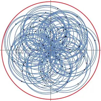
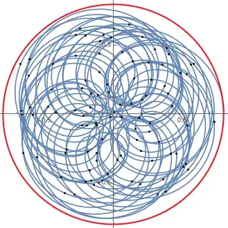
^{The black dots correspond to the integer values of $r$, the blue line gives the value of $F_r$ for the real values in-between, and the red circle has radius $1-\sqoverlap{\mu}{\lambda}$. Only values of $r$ between $1$ and $100$ are shown.}

Plotting even more points (all $r$ between $1$ and $10^3$), we see that the circle is essentially filled:

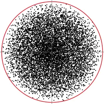
This is telling us that, in the general case, all we can say about $F_r$ is that it satisfies $$ |F_r|\le1-\sqoverlap\mu\lambda. $$ Now, to get the probability of finding the initial state $\ket\mu$ unchanged after $r$ applications of $U$, we need to study the quantity $|\langle\mu|U^r|\mu\rangle|=\big|\sqoverlap\mu\lambda+F_r\big|$. When $\sqoverlap\mu\lambda\ge1/2$ we know that $|F_r|\le\sqoverlap\mu\lambda$, and we thus have the bound $$ (2\sqoverlap{\mu}{\lambda}-1)^2 \le |\langle\mu|U^r|\mu\rangle|^2 \le 1,\quad \forall r. $$ On the other hand, when the initial squared overlap is smaller than $1/2$, we can have $F_r=-\sqoverlap\mu\lambda$, and thus we get the trivial bound $|\langle\mu|U^r|\mu\rangle|\in[0,1]$.

Putting the two cases together, if we plot the possible values of $|\langle\mu|U^r|\mu\rangle|^2$ as a function of $p\equiv\sqoverlap\mu\lambda$ we get the following:

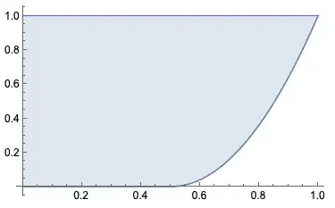
The interesting conclusion is that we can say something about the possible probabilities of a state remaining unchanged after a number of applications of the same unitary $U$, provided that the initial overlap between the state and one of the eigenvectors of $U$ is big enough. Let me remark a few other things here:

• There is no loss of generality in our initial assumption that the eigenvalue of some $\ket\lambda$ is $1$. We can repeat the same identical argument by just taking an arbitrary eigenvector of $U$ with eigenvalue $e^{i\varphi}$, by only replacing each instance of $U$ with $U e^{-i\varphi}$. Most notably, this does not affect the final result on $|\langle\mu|U^r|\mu\rangle|$.

• If $\sqoverlap\mu\lambda=1-\delta$ with $\delta\ge0$ small, then the bound can be simplified to $|\langle\mu|U^r|\mu\rangle|^2\ge 1-4\delta$.

• Because we are not putting any constraint on $U$ or $r$ other than the initial overlap $\sqoverlap\mu\lambda$, we can also understand this result as telling us about the probability of $\ket\mu$ being unchanged upon a single application of a unitary $U$, or more generally about the probability of $\ket\mu$ being unchanged upon arbitrary applications of arbitrary unitaries all having an eigenvector close enough to $\ket\mu$.

---

Mathematica code to generate the plots of $F_r$:

dim = 5;
probs = 0.8 * # / Total @ # & @ RandomReal[{0, 1}, dim];
phases = RandomReal[{0, 2 Pi}, dim];
otherFactor[probs_, phases_, r_] := Total[Exp[I r phases] probs];
Show[
 ParametricPlot[ReIm@otherFactor[probs, phases, r], {r, 0, 100}, 
  PlotPoints -> 60, MaxRecursion -> 10, 
  PlotRange -> ConstantArray[{-.9, .9}, 2]],
 Graphics[{ 
   Point@Table[ReIm@otherFactor[probs, phases, r], {r, 1, 100}],
   Thick, Red, Circle[{0, 0}, 0.8]
   }]
 ]