I am working on a model in superconductivity and have found the normal and anomalous Green's functions in real space. First, I computed the Green's functions in terms of the variables $ x $ and $ y $, then defined $ r = \sqrt{x^2 + y^2} $. After that, I used the flattening method to convert my Green's function to 1D for plotting, similar to what was done in Kim, J's paper. However, my professor said that this numerical method for converting 2D to 1D ruins our problem.
Instead, he suggested using polar coordinates $ (r, \theta) $, where $ x = r \cos\theta $ and $ y = r \sin\theta $. He advised me to plot the Green's function for some fixed values of $ \theta $. He also mentioned that he expects the concurrence to exhibit convexity and concavity for different values of $ \theta $.
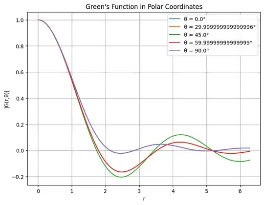
and I implement his suggestion . the visualization for Normal Green's function 
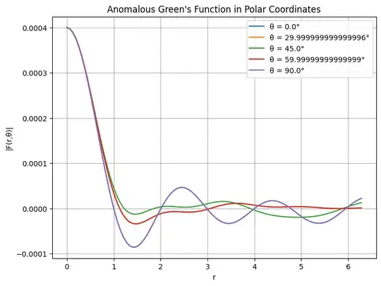
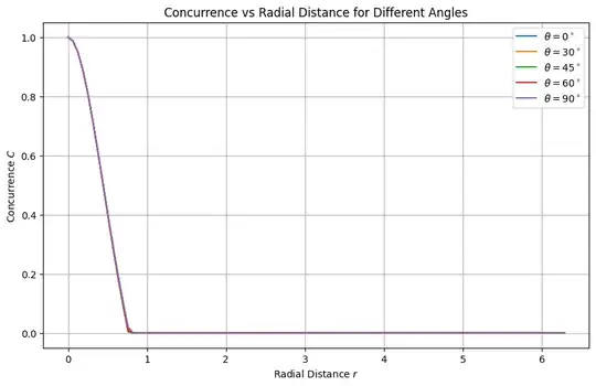
I see that for some specific values of $ \theta $, the normal Green's function $ G $ and the anomalous Green's function $ F $ are different. However, the concurrence appears to be the same for all of them.
and I have used these formula for compute the concurrence
$$f(r) = \frac{F(r)}{G(0)}$$ $$g(r) = \frac{G(r)}{G(0)}$$
- $ G(0) $ is the Green’s function at $ r = 0 $.
Compute $ p(r) $
$$ p(r) = \frac{f^2 + g^2}{2 + f^2 - g^2} $$
Compute the concurrence $ C(r) $
$$
C(r) = \max\left(0, \frac{3p - 1}{2}\right)
$$
I did not observe any convexity or concavity in my concurrence, and I did not see any differences in concurrence for these values of . However, the Green's functions differ for different .
Does anyone know why using the flatten method in Python to convert a 2D Green's function to 1D ruins my problem? Also, why does the concurrence remain the same for all $ \theta $ when I use polar coordinates, even though the Green's functions differ for different $ \theta $?

