Error graphs and how decoders perform matching on them?

Question

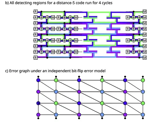
My understanding of decoding in quantum error correction is as follows. Assume you have a code where a single data or ancilla error triggers two detectors (except at space and time boundaries).

1. Make a circuit composed of stabilizer measurements.

2. Back propagate any error that anticommutes with the measurement through the (Clifford) circuit as far back as possible before it hits some kind of reset operation.

3. From this, you get detecting regions. In the bulk, each part of the circuit contains exactly two detecting regions. On the boundaries, you have that each part of the circuit contains only one detecting region.

4. A detector error model consists of the following: Each detector is a node and the weight of an edge connecting two detectors depends on the probability of an error happening in their overlap region.

5. Finally, when we run the circuit, the MWPM decoder sees which nodes have lit up (they will be in pairs due to 3, except at the boundary) and it joins edges between them such that the total edge weight is minimized.

This is shown in this paper

My questions is the following and are probably a result of gaps in my understanding regarding both error correction and probability theory:

If two detectors are lit, then there are usually many paths (each corresponding to a different set of errors) that connect them. Do we care about this at all?

1. If yes, how do we compute the list of all possible error paths from the edge weights we computed in Step 4? If two nodes are lit in the second figure, I need to sum over many paths that connect them? How do I enumerate over all these paths and compute each path's weight?

2. Why do I sum over all paths if my output is going to be one specific error path (the minimum weight path) that results in the observed syndrome? Isn't the decoder's problem simply to find one set of edges such that the syndrome is explained by it and the weight of that sum is minimized?

Answer 1

If two detectors are lit, then there are usually many paths (each corresponding to a different set of errors) that connect them. Do we care about this at all?

Yes, some paths may flip the observable while others may not. For example, for the surface code, some paths may connect nodes to the boundary while other paths may connect nodes to each other. Observables are explained in Oscar Higgott's thesis or this paper on detector error models.

If yes, how do we compute the list of all possible error paths from the edge weights we computed in Step 4? If two nodes are lit in the second figure, I need to sum over many paths that connect them? How do I enumerate over all these paths and compute each path's weight?

Three questions, so three answers:

1. This usually isn't done as it is too slow. Belief propagation doesn't compute edge weights of error paths. Minimum-weight perfect matching uses Dijkstra's algorithm to calculate the path with the minimum weight.
2. No you don't need to.
3. You can find all paths and then one by one compute the weights of each path.

Why do I sum over all paths if my output is going to be one specific error path (the minimum weight path) that results in the observed syndrome? Isn't the decoder's problem simply to find one set of edges such that the syndrome is explained by it and the weight of that sum is minimized?

1. You don't sum over all paths.
2. This question is unclear to me. The path the decoder chooses does matter as some paths may flip the observable.

Answer 2

In its initial formulation, the Minimum-Weight Perfect Matching decoder does not pair syndrome excitations directly in the graph associated to the detector error model.

Looking at the Wikipedia entry for a perfect matching, a perfect matching in a graph $G$ is a set of edges of $G$ such that any vertex of $G$ is incident to exactly one of these edges. Thus, a matching cannot include a path linking two excited nodes and will rarely be perfect if performed directly on the graph associated to the detector error model.

The perfect matching is sought in a different graph: a complete graph (thus guaranteeing the existence of a perfect matching) which has a vertex for each excited node of the syndrome. The edge linking two of these vertices will have a weight depending on the likelihood of a chain of errors to happen between the two detection events. How the weight associated to each edge is computed will vary depending on the decoder you use. Finding a perfect matching in a graph can be done efficiently thanks to the blossom algorithm.

If you were to use the Maximum Likelihood Decoder, you would be looking for the most probable equivalence class of errors, so the weights would have to depend on the probability of all the possible paths linking your two detection events. This is a huge task, since you have to repeat it for each possible pair of detection events for your complete graph. That is why the Maximum Likelihood decoder is not practical: the weights cannot be efficiently computed.

In the traditional MWPM decoder, the weight is set to the most probable chain of errors linking the two detection events. Computing this weight is equivalent to computing the shortest path that connects these detection events in the error graph. Shortest paths can be efficiently computed, so the MWPM decoder is practical. If the shortest path you identified would cross a logical observable, then the decoder will decide that this observable has been flipped when the associated edge in the complete graph belongs to a matching.

As @CraigGidney mentionned, the explicit use of the complete graph is not the state of the art anymore (see the newest Pymatching paper), one can directly pair the detection events in the error graph to save time. The deduced pairings would correspond to a perfect matching of minimum weight in the complete graph.