Numerical integration of Schrödinger equation with Pennylane

Question

I am trying to make a sort of Rabi experiment with Pennylane pulse module, using as hamiltonian the qml.pulse.transmon_interaction and driving qml.pulse.transmon_drive with constant amplitude. I have seen some weird behaviour. Let me first show you my code:

import pennylane as qml
import jax
from jax import numpy as jnp
import matplotlib.pyplot as plt
w0 = 1 / (2 * jnp.pi)
w1 = 3 / (2 * jnp.pi)
g = 0.1 / (2 * jnp.pi)
amp = lambda A, t: A
phase = lambda phi0, t: phi0
ham = qml.pulse.transmon_interaction(qubit_freq=[w0, w1], connections=[[0,1]], coupling=g, wires=[0,1])
ham += qml.pulse.transmon_drive(amplitude=amp, phase=phase, freq=w0, wires=0)
dev = qml.device("default.qubit", wires=range(2))
@jax.jit
@qml.qnode(dev, interface="jax")
def qnode(params, duration):
    qml.evolve(ham)(params, duration)
    return qml.expval(qml.PauliZ(0)), qml.expval(qml.PauliZ(1))
def rabi_oscillations(time_duration: float, max_amplitude: float):
    phi0 = 0
    func = jax.vmap(qnode, in_axes=(0,0))
    As = jnp.linspace(1e-2, max_amplitude, 100)
    durations = time_duration * jnp.ones_like(As)
    params = jnp.stack([As, jnp.full_like(As, phi0)], axis=-1)   # [[As[0], phi0], [As(1), phi0], ...]
z0s, z1s = func(params, durations)
plt.plot(As, z0s, label='z0s')
plt.plot(As, z1s, label='z1s')
plt.legend()

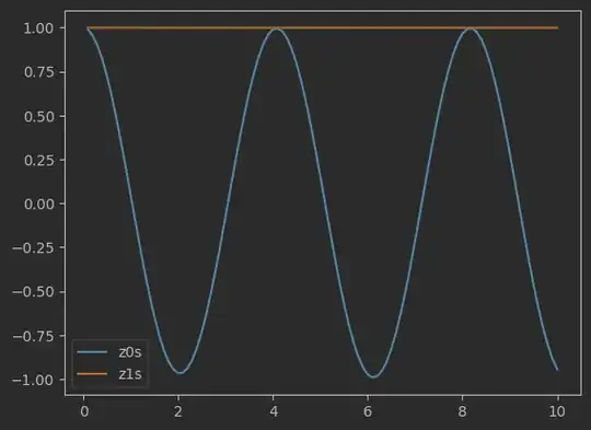
The idea was just to act on qubit 0 while qubit 1 is at rest, and see how the Rabi oscillations are. As suggested by some bibliography I have seen, I took $|\omega_1 - \omega_2| \gg g$ to avoid interaction between qubits. I should then see how expected value of qubit 1 is constant ($|0\rangle$) while qubit 0 suffers a $X$ rotation, whose angle is basically $A \cdot T$ being $T$ the pulse duration.

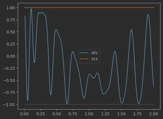
This is the case when I do: rabi_oscillations(time_duration=0.5, max_amplitude=10):

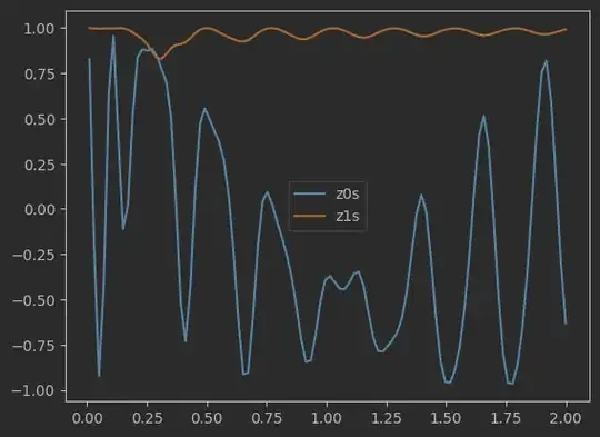
But things mess up if I increase time duration, for instance rabi_oscillations(time_duration=10, max_amplitude=2):

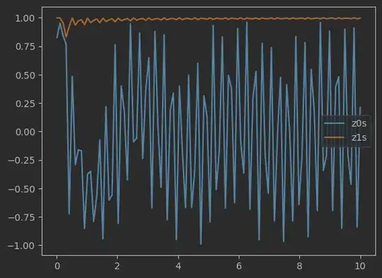
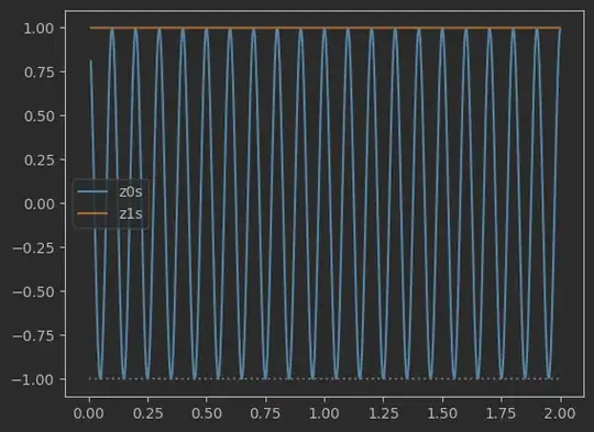
or decreasing the amplitude range:

I have been searching in the qml.evolve documentation and source code and I see that the differential equation is solve with scipy.integrate.odeint function, so qml.evolve admits some kwargs. Among them , atol is supposed to control the absolute error tolerance. I think this non-sense plot has to do with numerical approximation precision, since if I do qml.evolve(ham)(params, duration, atol=atol) inside the qnode function, I get different results. However, I do not suceed at controlling it, and do not understand its behaviour.

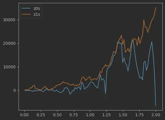
According to ParametrizedEvolution Pennylane class (which is in charge for solving the Schrödinger evolution when calling qml.evolve), the default value is 1.4e-8. If I decrease this tolerance, I do not get a different plot than the ones I displayed above (I did up to atol=1e-20). I think that very small values of atol mess things up even more, since atol=1-30 returns nan for z0s and z1s arrays, and atol=1e-25 returns some nan values as well. However, I am sure changing atol has some effects on solutions because setting atol=1e-4 returns awful solutions (probabilities beyond 1):

I also played a bit with rtol parameter but it seems to have no effect at all. hmax and mxstep arguments default to ´np.inf´, which I think that gives the best accuracy. I think there is not much I can do with numerical integration from my side.

As conclussion, I think that or I manually change the numerical integration function or that the problem has nothing to do with it. But in the latter, I cannot explain the results. Maybe some of you could help me since I am stuck :(

Answer 1

I am not 100% sure about this, so please double-check me, but I am pretty sure this is not a numerics problem but a physics problem. You can crank up the numbers for numerical accuracies (and in some cases above you should actually increase them) and get consistent behavior.

So first of all and most importantly, what you are simulating is not a pure Rabi oscillation. The transmon_interaction term contains both $\propto \omega_q Z_q$ and $\propto g_{qp} X_q X_p$. You are neglecting the latter one by setting g very small, but there is still the first term! So while the transmon_drive term ($\propto Y$) rotates the qubit amplitude around the Y axis, but at the same time you still have the precision of the qubit around Z at its own resonance frequency.

Now you chose a setup where you are simulating the pulse for a fixed period of time and vary the interaction strength, so depending on the interplay between amplitude and time, you arrive at different points on the bloch sphere in your plot, wouldnt that explain why you get no pure Rabi oscillation, in particular when the time duration is much longer?

If you really want to simulate just pure Rabi oscillations, I think the best thing to do would be to go to the rotating frame of qubit 0 (this will then just result in something like a $e^{i t Y}$ evolution, almost trivially. (see eq. (79) and the following in 1904.06560)

In terms of accuracy, beside the atol and rtol arguments you already found, you can also force the integrator to take more steps by feeding it an array of time-steps that it then needs to evaluate on. Also you should increase the number of amplitude points when the behavior is more oscillatory.

Let me know if this helps!

Answer 2

I think I found the solution myself thanks to @Korbinian Kottmann answer. Let me explain it while answering its post:

I know it is not a pure Rabi Oscillation, however, I think it can be considered as so. As Korbinian said, I can neglect the interacting term part of the Hamiltonian (the one containing the kronecker product of ladder operators) since I chose a proper $g$, so it remains a $\sigma_i^Z$ term for each qubit.

However, as I chose a pulse frequency exactly as qubit 0 natural frequency, this term vanishes on the driving rotating frame (equation 92 of the same reference Korbinian cited). In this equation, as the phase is chosen to be $\phi=0$, the remaining term is just a $\sigma_i^Y$ (sorry, on my question I accidentally said $X$ rotation), so in this frame I can neglect the $Z$ rotation Korbinian mentioned. And as this frame is obtained applying a unitary operator: $U=e^{ i \omega_d t \sigma_0^Z /\hbar}$ where $\omega_d$ is the driving frequency, and this unitary operator commutes with $\sigma_0^Z$ and $\sigma_1^Z$, the measurement of $\sigma_i^Z$ operators is equivalent in both frames $$\langle \sigma_1^Z \rangle_{|\psi\rangle} = \langle \psi |\sigma_i^Z | \psi\rangle = \langle \psi |U^\dagger U\sigma_i^Z | \psi\rangle = \langle \psi U^\dagger| \sigma_i^Z | U \psi\rangle = \langle \sigma_1^Z \rangle_{|\tilde \psi\rangle},$$ where $|\tilde \psi \rangle$ denotes the quantum state evolving according to transformed hamiltonian.

Considering this, I could explain the little perturbations that qubit 1 suffers deviating it from $|1\rangle$ state, since as Korbinian said, this qubit indeed suffers a $Z$ rotation (I am not applying a driving to it, so the $Z$ does not vanish now), but regarding qubit 0, the evolution must be a $Y$ according to my reasonment, which is clearly not in the plots I uploaded. The only things that could explain some differences to perfect $Y$ rotations could be: a) $g$ is not small enough and there is a reamining interaction I must consider (I would be shocked if the oscillations are like the ones I get, interferring qubit 0 so much and qubit 1 that little). b) Equation (92) is obtained performing a Rotating Wave Approximation, relying on the fact that $\omega_d + \omega_0 \gg |\omega_d - \omega_0|$. From the numbers I used, this means considering $4 \gg 0$ (which might be too pretentious).

Regarding a), I decreased $g$ to g = 1e-5 / (2 * jnp.pi) and I stil get crazy behaviour of qubit 0 (and now qubit 1 is not perturbed). Here is the corresding evolution ( rabi_oscillations(time_duration=10, max_amplitude=2)):

Regarding b), I changed $\omega_0$ to w0 = 100 / (2 * jnp.pi) (keeping g = 0.1 / (2 * jnp.pi) as before) and run rabi_oscillations(time_duration=10, max_amplitude=2) getting good oscillations now:

Additionally, the qubit 1 perturbation is now gone. So it results it is just a matter of not satisfying RWA conditions.

Thank you, Korbian, it really helped me your contribution. Please, I would be pleased if you could answer me and tell me if you agree or not with my proposed solution.