Are concurrence $C$ and purity of reduced state $p$ related by $C^2\le 4p(1-p)$?

Question

Asking this question to an AI, I got the result that the relation between concurrence and purity of a single qubit in a mixed bipartite state, as follows:

$$C^2 \le 4p(1-p)\,, $$

Where $C$ is concurrence, and $p$ is the purity of a single qubit.

Unfortunately, AI didn't give any resources. I want resources that refer to this inequality.

glS · Accepted Answer · 2024-03-21T19:49:06.540

The source is that it probably just made it up. Funnily enough, chatgpt3.5 also gives me the same relation if asked in general for an "inequality between concurrence and purity of reduced state". To then come up with a made up reference (the reference kind of exists, but certainly doesn't contain what gpt3.5 says it does, see https://i.sstatic.net/hOABE.png; it also keeps changing both inequality and "source" if reasked so... yes, it just made the whole thing up).

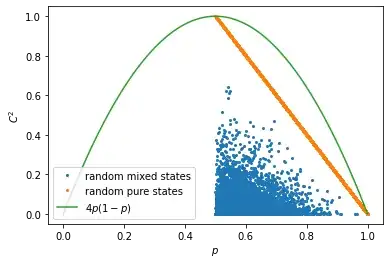
That said, it does seem to hold at least for two-qubit states. Note that for pure states the concurrence is defined as such that $C^2=2(1-p)$ with $p=\operatorname{tr}(\rho_A^2)$ with $\rho_A\equiv\operatorname{tr}_B(\rho)$. And obviously $2(1-p)\le 4p(1-p)$ for all $p\in[1/2,1]$. For mixed states the concurrence is defined via convex roof extension so if it holds for pure states I think it has to hold for all mixed states as well.

I should add though that it's a completely useless (if true) inequality. You might as well just use $C^2\le 2(1-p)$ which is easier and tighter.

Here's a some quick and dirty numerics of how the quantities are related:

Generated with

    import numpy as np
    import matplotlib.pyplot as plt
    import qutip
    num_states = 10000
    # initialise a table of real numbers to store the purity and concurrence
    data = np.zeros((num_states, 2))
    for idx in range(num_states):
        dm = qutip.rand_dm(N=4, dims=[[2, 2], [2, 2]])
        # purity of the reduced state
        purity = dm.ptrace(0).purity()
        concurrence = qutip.concurrence(dm)
        data[idx] = [purity, concurrence]
    # same thing but with random PURE states
    data_pure = np.zeros((num_states, 2))
    for idx in range(num_states):
        dm = qutip.rand_dm(N=4, dims=[[2, 2], [2, 2]], pure=True)
        # purity of the reduced state
        purity = dm.ptrace(0).purity()
        concurrence = qutip.concurrence(dm)
        data_pure[idx] = [purity, concurrence]
    # plot the data in `data` together with the C^2=4p(1-p) curve with p purity and C concurrence
    fig, ax = plt.subplots()
    ax.plot(data[:, 0], data[:, 1]**2, 'o', markersize=2, label='random mixed states')
    ax.plot(data_pure[:, 0], data_pure[:, 1]**2, 'o', markersize=2, label='random pure states')
    p = np.linspace(0, 1, 100)
    ax.plot(p, 4*p*(1-p), label=r'$4p(1-p)$')
    ax.set_xlabel(r'$p$')
    ax.set_ylabel(r'$C^2$')
    ax.legend()
    plt.show()

Are concurrence $C$ and purity of reduced state $p$ related by $C^2\le 4p(1-p)$?

1 Answers1