Plotting Fisher Information using PennyLane

Question

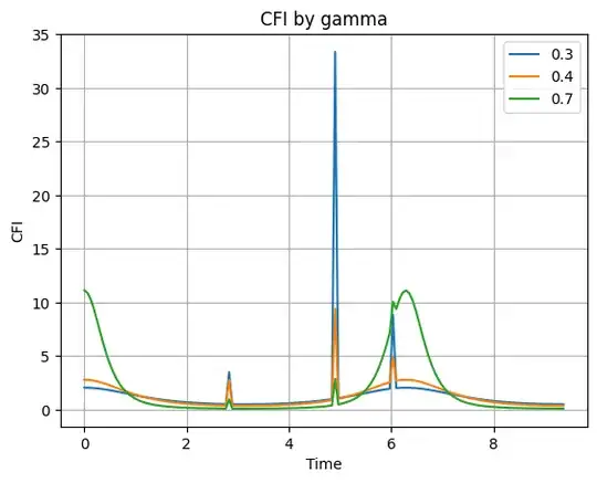
I made 2-qubit based circuit with post-selection method.

Post-selection method is, Let $$ K = \begin{bmatrix} \sqrt{1-\gamma} & 0 \\ 0 & 1 \end{bmatrix}\,. $$

Then, $$ \rho_{\text{post-selection}} = \frac{(K \otimes K) \rho (K^{\dagger} \otimes K ^{\dagger})} {Tr\big[(K \otimes K) \rho (K^{\dagger} \otimes K ^{\dagger})\big]} \,.$$

With the above density matrix, I calculated Classical Fisher Information with PennyLane's qml.qinfo.classical_fisher for the selected sweeping boundary 0 ~ 3$\pi$. Using that data, I created a plot for 3 cases of $\gamma = \{0.3, 0.4, 0.7\}$ using plt.plot

However, the result of 3-gamma with the selected sweeping area shows a distorted shape whereas it should be smooth. I noticed significant distortion at Time: around 5~

Can anybody help with this? Thanks in advance

import pennylane as qml
from pennylane import numpy as np
from IPython.display import display, Latex
import numpy as np_
import scipy as sp
import matplotlib.pyplot as plt
2-qubit
dev = qml.device('default.mixed', wires= 2)
== Hamiltonian setup ==
coeffs = [1]
obs = [qml.PauliZ(0) @ qml.PauliZ(1)]
hamiltonian = qml.Hamiltonian(coeffs, obs)
Tau_global, Phi_global = np.zeros(3), 0
Gamma_ps_global = 0
1-layer
@qml.qnode(dev)
def circuit_alt(phi_in):
    global Tau_global, Phi_global
theta_init, tau_1, tau_2,  = [1e-3]*3
phi = phi_in

# Stage_1: RY for pi/2
qml.RY(np.pi/2, wires=0)
qml.RY(np.pi/2, wires=1)

# Stage_2: Entangler    
qml.ApproxTimeEvolution(hamiltonian, -tau_1/2, 1)

qml.RX(theta_init, wires = 0)    
qml.RX(theta_init, wires = 1)    

qml.RY(-np.pi/2, wires = 0)    
qml.RY(-np.pi/2, wires = 1)   

qml.ApproxTimeEvolution(hamiltonian, -tau_2/2, 1)

qml.RY(np.pi/2, wires = 0)    
qml.RY(np.pi/2, wires = 1) 

# Stage_3: Accumulator
qml.ApproxTimeEvolution(hamiltonian, -phi/2, 1)


qml.RY(-np.pi/2, wires=0)
qml.RY(-np.pi/2, wires=1)

return qml.density_matrix(wires=[0, 1])


fig, ax = qml.draw_mpl(circuit_alt)(0)
@qml.qnode(dev)
def Post_selection_alt(phi):
    global Gamma_ps_global
    Gamma_ps = Gamma_ps_global
# Get density matrix from circuit_alt
density_matrix = np.zeros((4, 4), dtype=np.complex128)
density_matrix = circuit_alt(phi)

qml.QubitDensityMatrix(density_matrix, wires=[0, 1])

# Kraus operator for 2*2 matrix
K = np.array([ [np.sqrt(1 - Gamma_ps), 0], [0, 1] ])
K_H = K.conj().T

Numerator = sp.linalg.kron(K, K) @ density_matrix @ sp.linalg.kron(K_H, K_H)
Denominator = np.trace(sp.linalg.kron(K, K) @ density_matrix @ sp.linalg.kron(K_H, K_H))

rho_ps = Numerator / Denominator

qml.QubitDensityMatrix(rho_ps, wires=[0, 1])

return qml.density_matrix(wires=[0, 1])



def Sweep(Sweep_bound, Gamma_ps_in):
PHI = np.arange(Sweep_bound[0], Sweep_bound[1], Sweep_bound[2]).reshape(-1, 1)

Data = np.zeros((len(PHI), 1 + len(Gamma_ps_in)))

Data[:, 0] = PHI.squeeze()

GAMMA_INDEX_IN_DATA = 1

global Gamma_ps_global


for Gamma_index in range(len(Gamma_ps_in)):
    Gamma_ps_global = Gamma_ps_in[Gamma_index]

    for i in range(len(PHI)):
        Data[i][Gamma_index + GAMMA_INDEX_IN_DATA] = qml.qinfo.classical_fisher(Post_selection_alt)(PHI[i])


return Data



Sweep_data = np_.array([1e-4, np.pi * 3 + 1e-4, np.pi/(25*2)])
Gamma_ps_desired = 0.3, 0.4, 0.7, 0.8
Result = Sweep(Sweep_data, Gamma_ps_desired)
plt.plot(Result[:,0], Result[:,1], label = 0.3)
plt.plot(Result[:,0], Result[:,2], label = 0.4)
plt.plot(Result[:,0], Result[:,3], label = 0.7)
plt.title('CFI by gamma')
plt.xlabel('Time')
plt.ylabel('CFI')
plt.legend()
plt.grid()