I am struggling to understand why the lattice splitting procedure works precisely. I am following the appendix in this paper.
[edit]: While the answer in this topic answers the question, the concept that allows to properly understand the solution is solved in this topic How to find the stabilizer generators for a post-measurement state?
The context
I will focus on the merging for rough boundaries as represented in the image below.
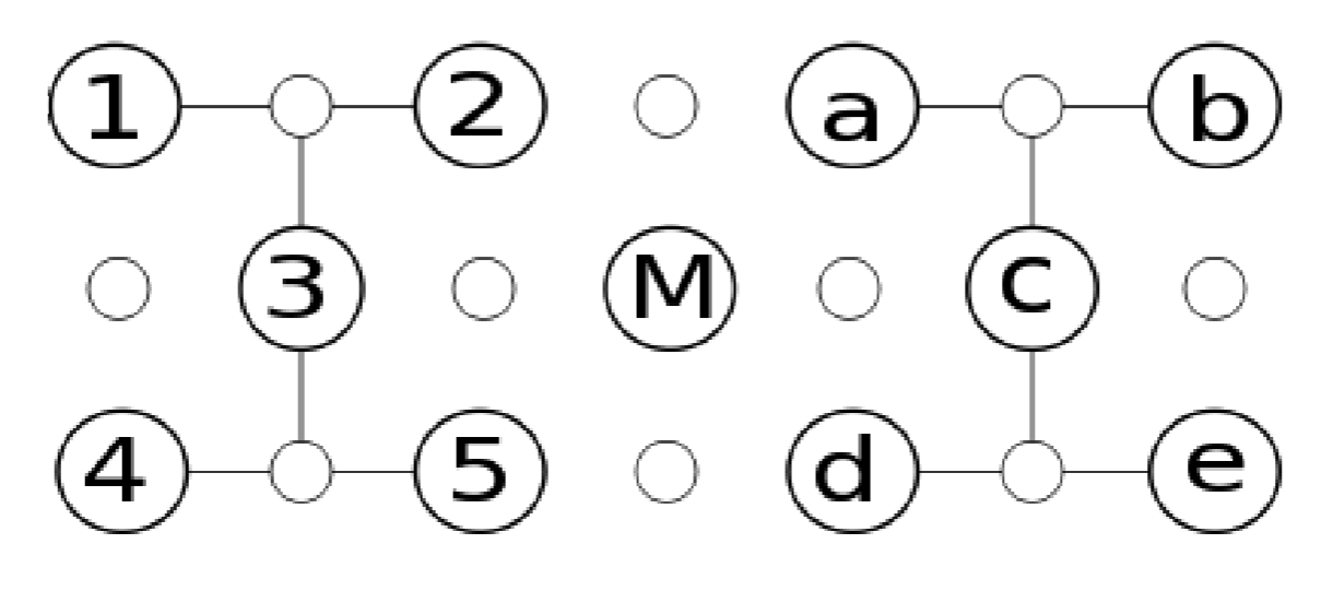
I assume that the total state at "time 0" is $|\psi\rangle=|0_L\rangle |0 \rangle |0_L\rangle$ where the first logical qubit is the one on the left surface, the middle one is the measurement qubit $M$ and the right one is the state stored on the right surface.
I need to show that after the lattice merging, which consists in "turning on" the $X$ stabilizers $X_2 X_a X_M$, $X_5 X_d X_M$, and in changing the $Z$ stabilizers: $Z_a Z_c Z_d \to Z_a Z_c Z_d Z_M$, $Z_2 Z_3 Z_5 \to Z_2 Z_3 Z_5 Z_M$, the state at the end of the procedure will become $|\psi \rangle \to |0_L\rangle$ which is the logical $0$ of the now merged surface. Here I only described "which stabilizer changed", but of course we will have all along many other "stabilizers" activated, $Z_1 Z_3 Z_4$ would be an example.
If I properly understand this example, by linearity I could understand what happens for arbitrary initial qubit stored on the two surfaces before merging (as the reasoning would be similar for any computational state).
My question
In the paper, it is said that before any merging, the stabilizers for $|0_L\rangle |0 \rangle |0_L \rangle$ are the following:
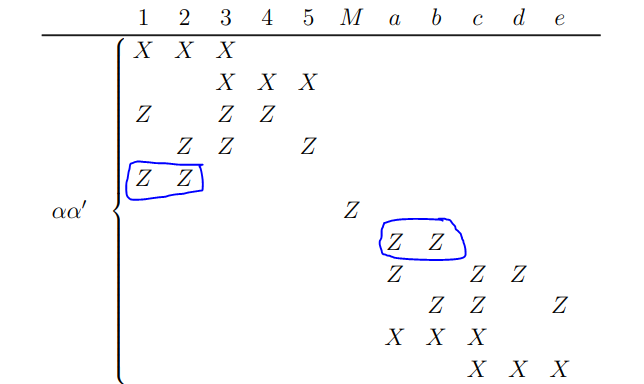
I agree with that. (don't pay attention to the blue lines right now).
Then, the authors reason sequentially. They consider first "turning on" $X_2 X_M X_a$ (and even if not explicitly written, they also do the change $Z_a Z_c Z_d \to Z_a Z_c Z_d Z_M$, $Z_2 Z_3 Z_5 \to Z_2 Z_3 Z_5 Z_M$. They obtain the following stabilizer table:
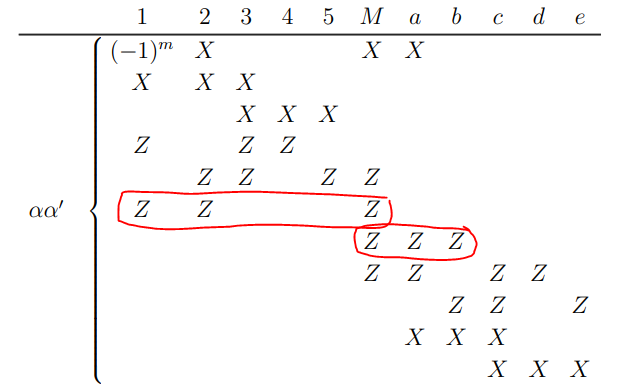
I agree with everything but the red lines. They are corresponding to the blue lines in the previous table (which represented stabilizers for the logical $|0_L\rangle$ for the two surfaces), but now multiplied by $Z_M$. Indeed, I remind that the logical $Z$ for the first and second surfaces can be written as $Z_1 Z_2$ and $Z_a Z_b$ respectively.
I understood the presence of the blue lines in the previous table. Even though we were not "actively" measuring the associated Pauli, the state was by definition an eigenstate of those. However, I don't understand the red lines in the second table, and this for the following two reasons:
- We are not actively measuring $Z_1 Z_2 Z_M$ neither $Z_a Z_b Z_M$.
- Even if we are not actively measuring those, nothing tells us that the state would be an eigenstate of those two operators. If it appears to be the case I don't find it obvious and it would have to be shown.
In conclusion: could someone explain to me why the red lines are present in the second table? If I understand this I guess I could understand the rest of the proof yielding to $|\psi \rangle \to |0_L \rangle$