Do entangled measurements across multiple copies help in state distinguishability?

Question

Consider two density matrices $\rho$ and $\sigma$. The task is to distinguish between these two states, given one of them --- you do not know beforehand which one.

There is an optimal measurement to distinguish between these two states --- the Helstrom measurement. Note that it is an orthogonal projector.

Now, if we have $k$ copies of the states, do we get any advantage from an entangled measurement across $k$ copies?

The optimal measurement, in this case, is a Helstorm measurement once again, of $\rho'$ and $\sigma'$, with $\rho' = \rho^{\otimes k}$ and $\sigma' = \sigma^{\otimes k}$. In general, this is an entangled measurement across the $k$ copies.

If we measure each copy separately and do some quantum or classical post-processing afterwards, how close can we go to the optimal distinguishing probability?

glS · Accepted Answer · 2021-09-28T13:31:18.227

Very roughly speaking, yes, "entangled measures" (that is, global measures on multiple copies) make it easier to distinguish states.

The intuitive reason is that, if $\langle\rho,\sigma\rangle\equiv\operatorname{Tr}(\rho\sigma)<1$, then $\langle\rho^{\otimes n},\sigma^{\otimes n}\rangle=\langle\rho,\sigma\rangle^n$, which decreases with increasing $n$. You can then see that in the limit $n\to\infty$, the states become orthogonal, and thus perfectly distinguishable.

For example, if you take $\rho=|0\rangle\!\langle0|$ and $\sigma=|+\rangle\!\langle+|$ and compute the trace norm $\|\rho^{\otimes n}-\sigma^{\otimes n}\|_1$ as a function of $n$ (which you'll remember from the linked post, and the discussion in this post, gives you the maximum distinguishing probability), you get

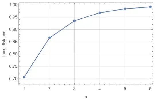
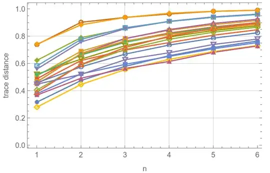
If you do the same for randomly generated three-dimensional states, you always get a similar behaviour:

To see that these better performance are made possible by entangled measures, consider again $\rho=|0\rangle\!\langle0|$ and $\sigma=|+\rangle\!\langle+|$. The corresponding Helstrom measurement is $$\Pi_\pm \equiv \mathbb P[(-1\pm \sqrt2)|0\rangle+|1\rangle], \qquad \mathbb P[|\psi\rangle]\equiv\frac{|\psi\rangle\!\langle\psi|}{\langle\psi|\psi\rangle}.$$ On the other hand, the Helstrom measurement corresponding to $\rho^{\otimes 2}-\sigma^{\otimes 2}$ is $$\Pi_\pm = \mathbb P[(-3\pm2\sqrt3)|00\rangle+|01\rangle+|10\rangle+|11\rangle],$$ which are clearly projections on entangled states.

The figures above were generated with the following MMA snippets:

KP[arg_] := arg;
KP[args___] := KroneckerProduct[args];
traceDistance[dm1_, dm2_] := dm1 - dm2 // Eigenvalues // Abs // Total // #/2 &;
With[{rho = {{1, 0}, {0, 0}}, sigma = {{1, 1}, {1, 1}}/2},
  Table[
    traceDistance[KP @@ ConstantArray[rho, n], KP @@ ConstantArray[sigma, n]],
    {n, Range@6}
  ] // ListPlot[#,
    Joined -> True, PlotMarkers -> Automatic, 
    GridLines -> Automatic, PlotRange -> All, Frame -> True, 
    FrameLabel -> {"n", "trace distance"}] &
 ]

and

KP[arg_] := arg;
KP[args___] := KroneckerProduct[args];
traceDistance[dm1_, dm2_] := dm1 - dm2 // Eigenvalues // Abs // Total // #/2 &;
randomDM[dim_Integer] := RandomComplex[{-1 - I, 1 + I}, {dim, dim}] // Dot[#, ConjugateTranspose@#] & // #/Tr@# &;
data = Table[
  With[{rho = randomDM@3, sigma = randomDM@3},
    Table[
      {n, traceDistance[KP @@ ConstantArray[rho, n], KP @@ ConstantArray[sigma, n]]},
      {n, Range@6}
    ]],
  20
];
ListPlot[data,
  Joined -> True, PlotMarkers -> Automatic, 
  GridLines -> Automatic, PlotRange -> All, Frame -> True, 
  FrameLabel -> {"n", "trace distance"}
]

Do entangled measurements across multiple copies help in state distinguishability?

1 Answers1