Hadamard Overlap Test

Question

I am trying to understand a test called Hadamard Overlap Test, which consists of a destructive swap test (section IV of swap test and Hong-Ou-Mandel effect are equivalent) right after a Hadamard test. The circuit is from the Variational Quantum Linear Solver paper:

The authors claim that "conditioning the measurement on the ancilla qubit to yield the $|\boldsymbol{0}\rangle$ state, we can perform the depth-two Overlap circuit between registers S1 and S2 to get": \begin{equation} \begin{aligned} P(0) &=\frac{1}{2}\left(\left\langle\mathbf{0}\left|U^{\dagger} V\right| \mathbf{0}\right\rangle\left\langle\mathbf{0}\left|V^{\dagger} U\right| \mathbf{0}\right\rangle\right.+\left\langle\mathbf{0}\left|U^{\dagger} A_{l^{\prime}} A_{l} V\right| \mathbf{0}\right\rangle\left\langle\mathbf{0}\left|V^{\dagger} A_{l}^{\dagger} A_{l^{\prime}}^{\dagger} U\right| \mathbf{0}\right\rangle \\ &\left.+\operatorname{Re}\left[\left\langle\mathbf{0}\left|U^{\dagger} A_{l} V\right| \mathbf{0}\right\rangle\left\langle\mathbf{0}\left|V^{\dagger} A_{l^{\prime}}^{\dagger} U\right| \mathbf{0}\right\rangle\right]\right) \end{aligned} \end{equation}

$|\boldsymbol{0}\rangle$ represents a vector of 0 qubits, those making up the registers $S_1$ or $S_2$. I can't understand how to derive this result. In particular, I have the following questions:

• What are we exactly measuring by $P(0)$? From the circuit, it seems like all the qubits are measured, and that is also the case when you do a swap test according to the reference above. I initially thought that $P(0)$ is the probability of getting 0 in the ancilla, but this should not be the case, because otherwise what is the effect of the CNOT and H performed? What I mean is that the gates inside the box are not controlled on the ancilla, so they cannot change the outcome of the ancilla.
• How do you get to this result? Below is my attempt and what I achieved so far

\begin{equation} \begin{aligned} & |0 \rangle |\boldsymbol{0} \rangle |\boldsymbol{0} \rangle \xrightarrow{V, U} |0 \rangle V|\boldsymbol{0} \rangle U|\boldsymbol{0} \rangle \xrightarrow{H}\frac{1}{\sqrt{2}}\left(|0 \rangle +|1 \rangle \right)V|\boldsymbol{0} \rangle U|\boldsymbol{0} \rangle \xrightarrow{A_l, A_{l'}^{\dagger}}\\ &\frac{1}{\sqrt{2}}\left(|0 \rangle V|\boldsymbol{0} \rangle U|\boldsymbol{0} \rangle +|1 \rangle A_lV|\boldsymbol{0} \rangle A_{l'}^{\dagger}U|\boldsymbol{0} \rangle \right) \xrightarrow{H}\\ & \frac{1}{2}\left[|0 \rangle(V|\boldsymbol{0} \rangle U|\boldsymbol{0} \rangle +A_lV|\boldsymbol{0} \rangle A_{l'}^{\dagger}U|\boldsymbol{0} \rangle )+|1 \rangle (V|\boldsymbol{0} \rangle U|\boldsymbol{0} \rangle -A_lV|\boldsymbol{0} \rangle A_{l'}^{\dagger}U|\boldsymbol{0} \rangle )\right] \end{aligned} \end{equation} Now, one measures the ancilla, if it results in a 0 state, the system collapses in \begin{equation} \frac{1}{2}(V|\boldsymbol{0} \rangle U|\boldsymbol{0} \rangle +A_lV|\boldsymbol{0} \rangle A_{l'}^{\dagger}U|\boldsymbol{0} \rangle) \end{equation} How does one implement the the CNOTs and H now? What are the further steps that yields the results of the authors?

Answer 1

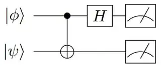
The missing step corresponds to the so-called Destructive Swap Test, which allows to compute the fidelity $|\langle \psi | \phi \rangle|^2$ between two $n$-qubit states $|\phi \rangle$ and $|\psi \rangle$ with a depth-2 circuit (on top of the preparation of $|\phi \rangle$ and $|\psi \rangle$ in parallel). For the sake of simplicity, I will first consider the $n = 1$ case, as the extrapolation to arbitrary $n$ is straightforward.

The fidelity between single-qubit states $|\phi \rangle$ and $|\psi \rangle$ is equal to the expectation value of the SWAP gate with respect to the state $|\phi \rangle \otimes |\psi \rangle$:

$(\langle \phi| \otimes \langle \psi |) \; \textrm{SWAP} \; (|\phi \rangle \otimes |\psi \rangle) = (\langle \phi| \otimes \langle \psi |) (|\psi \rangle \otimes |\phi \rangle) = \langle \phi | \psi \rangle \langle \psi | \phi \rangle = |\langle \phi | \psi \rangle|^2$.

The key idea behind the Destructive Swap Test corresponds to the following circuit identity:

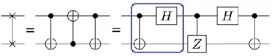
In words, the SWAP gate is equal to the diagonal matrix CZ up to a similarity transformation $\textrm{SWAP} = U^{\dagger} \; CZ \; U$, where $U$ corresponds to the subcircuit shown inside the blue box. Hence, we can compute the expectation value of SWAP by executing the following circuit

and associating $+1$ with all trials that yield $00$, $01$ and $10$, and $-1$ with all trials that yield $11$, as in $\textrm{CZ} = \textrm{diag}(1,1,1,-1)$. More concretely, the computed expectation value is

$\textrm{Tr}(\textrm{CZ} \; U(|\phi \rangle \otimes |\psi \rangle) (\langle \phi | \otimes \langle \psi |) U^{\dagger}) = \textrm{Tr}([U^{\dagger} \; CZ \; U] (|\phi \rangle \otimes |\psi \rangle) (\langle \phi | \otimes \langle \psi |)) = \textrm{Tr}(\textrm{SWAP} (|\phi \rangle \otimes |\psi \rangle) (\langle \phi | \otimes \langle \psi |)) = |\langle \phi | \psi \rangle|^2$.

The generalization to an arbitrary number of qubits $n$ for each register encoding the $n$-qubit states $|\phi \rangle$ and $|\psi \rangle$ simply corresponds to repeating this two-qubit circuit for all pairs of qubits of equal significance from each state. This corresponds to the last step of the circuit shown in the question, associated with the circuit inside the dashed line box.

Thus far, we have only considered separable states of the form $|\phi \rangle \otimes |\psi \rangle$. However, we can also consider its extension to the case where there is entanglement between the two $n$-qubit registers, which is the relevant case to answer this question. Suppose we have the following input state, $|\phi_1 \rangle \otimes |\psi_1 \rangle + |\phi_2 \rangle \otimes |\psi_2 \rangle$. The expectation value of the SWAP operator is

$\langle \textrm{SWAP} \rangle = (\langle \phi_1 | \otimes \langle \psi_1 | + \langle \phi_2 | \otimes \langle \psi_2 |) \; (|\psi_1 \rangle \otimes |\phi_1 \rangle + |\psi_2 \rangle \otimes |\phi_2 \rangle) = \langle \phi_1 | \psi_1 \rangle \langle \psi_1 | \phi_1 \rangle + \langle \phi_2 | \psi_2 \rangle \langle \psi_2 | \phi_2 \rangle + \langle \phi_1 | \psi_2 \rangle \langle \psi_1 | \phi_2 \rangle + \langle \phi_2 | \psi_1 \rangle \langle \psi_2 | \phi_1 \rangle$

This is precisely the result that we need to arrive at $P(0)$ stated above (cf. Eq. (C3) in reference paper). As derived in the statement of the question, the wave function encoded in S1 + S2 before this Destructive Swap Test and after the ancillary qubit is measured in $|0\rangle$ is

$\frac{1}{2} (V |0 \rangle \otimes U |0 \rangle + A_l V |0 \rangle \otimes A_{l'}^{\dagger} U |0 \rangle)$.

Hence, setting $|\phi_1 \rangle = \frac{1}{\sqrt{2}} V |0 \rangle$, $|\psi_1 \rangle = \frac{1}{\sqrt{2}} U |0 \rangle$, $|\phi_2 \rangle = \frac{1}{\sqrt{2}} A_l V |0 \rangle$ and $|\psi_2 \rangle = \frac{1}{\sqrt{2}} A_{l'}^{\dagger} U |0 \rangle$ in the previous equation for the entangled case yields the desired expression for $P(0)$, apart from a minor typo: The third term should have coefficient 1 (i.e., it should be outside the curved brackets), since $\textrm{Re}(a) = \frac{1}{2}(a + a^{*})$.

P.S.: The idea suggested by @DaftWullie of considering only the trials that yield all $2n+1$ qubits in state $|0\rangle$ could also be used to compute expectation values, but in this case it would not allow to avoid controlling the $U$ and $V(\alpha)$ subcircuits, which was the goal of the authors.

In this case, since all $2n$ qubits in the S1 and S2 registers are projected onto $|0\rangle$, the measured probability would be given by

$P' = |\langle \Phi^{+} | \frac{1}{2}(V |0 \rangle \otimes U |0 \rangle + A_l V |0 \rangle \otimes A_{l'}^{\dagger} U |0 \rangle )|^2,$

using once again the result derived at the end of the statement of this question. $|\Phi^{+} \rangle \equiv \frac{1}{\sqrt{2^n}} \sum_{j = 0}^{2^n-1} |j\rangle \otimes |j \rangle$ is just the state prepared by the circuit inside the dashed-line box of the figure in the question when acting on the fiducial state $|0 \rangle$. Now we can make use of the ricochet property of the $|\Phi^{+} \rangle$ state,

$(U \otimes V) |\Phi^{+} \rangle = (1 \otimes V U^{T}) |\Phi^{+} \rangle = (U V^{T} \otimes 1) |\Phi^{+} \rangle$

to express the probability as

$P' = |\langle \Phi^{+} | \frac{1}{2}(U^{T} V |0 \rangle \otimes |0 \rangle + U^{T} A_{l'}^{*} A_l V |0 \rangle \otimes |0 \rangle )|^2.$

At this point, we can plug the definition of $|\Phi^{+} \rangle$ into this expression to obtain

$P' = \frac{1}{4}|\frac{1}{\sqrt{2^n}} \sum_{i = 0}^{2^n - 1} \langle i |U^{T} V |0 \rangle \langle i |0 \rangle + \frac{1}{\sqrt{2^n}} \sum_{i = 0}^{2^n - 1} \langle i | U^{T} A_{l'}^{*} A_l V |0 \rangle \langle i |0 \rangle |^2 = \frac{1}{2^{n+2}} |\langle 0 | U^{T} V | 0 \rangle + \langle 0 | U^{T} A_{l'}^{*} A_l V |0 \rangle |^2 = \frac{1}{2^{n+2}} (|\langle 0 | U^{T} V | 0 \rangle|^2 + |\langle 0 | U^{T} A_{l'}^{*} A_l V |0 \rangle |^2 + 2 \textrm{Re}\{ \langle 0 | U^{T} V | 0 \rangle \; \langle 0 | V^{\dagger} A_{l}^{\dagger} A_{l'}^{T} U^{*} |0 \rangle \})$.

Clearly, the third term, which is the one that will remain once we subtract the probability associated with measuring the ancilla in $|1 \rangle$, does not quite yield the expectation values that the authors wished to compute. In principle, we could reformulate the circuit to have this third term in the form of the desired expectation value, but there is a caveat: The subcircuits $U$ and $V$ appear in different forms ($V$ / $V^{\dagger}$ and $U^{T}$ / $U^{*}$) in the two factors that multiply each other in the third term, so we would need to control $U$ and $V$ with the ancilla, which is precisely what the authors were trying to avoid in the first place.