I am not familiar with the specific notation in this paper, but I am very familiar with R. Featherstone's work.
It seems S9-S11 are the equations for the force and equipollent torque balance as applied to each body. And S14-S15 are the acceleration kinematics. Finally S16 is the joint condition as it related to the power through the joint (that is where the 0 on the right-hand side comes from). What is missing from the post to complete this endevour is the velocity kinematics and the rigid body dynamics equations.
And because the linked paper is by R.Featherstone who is best known for uitilizign "screw theory" in the dynamics of serially connected chains of bodies, I am going to try to explain how each equation is developed using vectors, but arrange the vectors in 6×1 groups that represent screws (twists and wrenches). You can use How is Screw Theory used in Robotics when you can do everything with regular kinematics? as a reference also.
Notation
Each vector quantity below is expressed along the common basis vectors of the inertial frame. The subscript indicates which body the quantity is associated with. Some quantities, such as torque, for example, require a reference point about which they are summed. This is indicated with a superscript when needed. If the superscript is omited then it is implied that the summation point is the "handle" of each body, which is the location of the pin joint as seen below.
Velocity kinematics
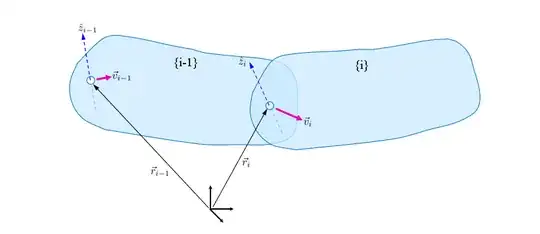
Consider two connected bodies, and we represent their motion by the motion of the handle (where the pin joint is located) $\vec{v}_i$ and the rotational motion of each body $\vec{\omega}_i$. Each pin has a hinge axis $\hat{z}_i$ and its relative rotational speed is $\dot{\theta}_i$.
We track the location of each pin joint with $\vec{r}_i$. The motion of the joint and thus the body is defined by the time derivative of this point $\vec{v}_i = \dot{\vec{r}}_i$.
Using the conventional vector form, we apply the velocity transformation rule $$\vec{v}_i = \vec{v}_{i-1} + \vec{\omega}_{i-1} \times ( \vec{r}_i - \vec{r}_{i-1}) \tag{1}$$
In addition, the rotational kinematics are established from the relative rotational velocity vector $\vec{\omega}_{\rm rel} = \hat{z}_i \dot{\theta}$ as $$ \vec{\omega}_i = \vec{\omega}_{i-1} + \hat{z}_i \dot{\theta} \tag{2}$$
See this post Absolute Angular Velocity - How to use? for proof of the above
But instead, if you use the velocity transformation rule to transform the quantities to the fixed origin of the inertial frame you will get the following set of equations
$$\begin{aligned}
\underbrace{\vec{v}_{i}+\vec{r}_{i}\times\vec{\omega}_{i}}_\text{motion of body i} & = \underbrace{ \vec{v}_{i-1}+\vec{r}_{i-1}\times\vec{\omega}_{i-1}}_\text{motion of body i-1} + \underbrace{ \vec{r}_{i}\times\hat{z}_{i} \dot{\theta}_i}_\text{relative motion} \\ \hline
\vec{\omega}_{i} &= \vec{\omega}_{i-1} + \hat{z}_{i} \dot{\theta}_i \end{aligned} \tag{3}$$
Using screw theory the two vector equations above are combined into a single twist equation for velocity kinematics
$$\boxed{\boldsymbol{v}_i = \boldsymbol{v}_{i-1} + \boldsymbol{s}_i \dot{\theta}_i} \tag{VK} $$
$$\begin{Bmatrix}\vec{v}_{i}+\vec{r}_{i}\times\vec{\omega}_{i}\\
\vec{\omega}_{i}
\end{Bmatrix} = \begin{Bmatrix}\vec{v}_{i-1}+\vec{r}_{i-1}\times\vec{\omega}_{i-1}\\
\vec{\omega}_{i-1}
\end{Bmatrix} + \begin{Bmatrix}\vec{r}_{i}\times\hat{z}_{i}\\
\hat{z}_{i}
\end{Bmatrix} \dot{\theta} $$
To understand the subtle change, instead of tracking the motion of a specific point attached to a body, we are measuring the velocity of whichever particle happens to pass over the origin at any instant, even if it isn't a physical particle, but a virtual location on the extended rotating frame of the body. It is like taking a magnifying glass and only looking at the origin as the body moves as only measuring the motion of the body at the origin.
This is exactly what the top vector in the screw above represennts and it is an invariant quantity for each body, meaning that at each instant $\vec{v}_{A}+\vec{r}_{A}\times\vec{\omega}=\text{<invariant>}$ regarless of which arbitrary point A used to track on the body.
An important quantity here, is the joint unit twist $$\boldsymbol{s}_{i}=\begin{Bmatrix}\vec{r}_i\times\hat{z}_{i}\\
\hat{z}_{i}
\end{Bmatrix}$$ which contains everything you need for the pivot in so-called Plucker coordinates of a line in space with direction $hat{z}_{i}$ that is passing through a point $vec{r}_i$. This quantity represents the relative axis of rotation between the two bodies.
Acceleration Kinematics
The time derivative of (3) gives us the acceleration kinematics between the two bodies, and to carry it out you need to know how to take derivatives on rotating frames (you can look it up) and you need to use the product rule of differentiation (a lot).
$$\begin{aligned}\dot{\vec{v}}_{i}+\vec{r}_{i}\times\dot{\vec{\omega}}_{i}+\vec{v}_{i}\times\vec{\omega}_{i} & =\dot{\vec{v}}_{i-1}+\vec{r}_{i-1}\times\dot{\vec{\omega}}_{i-1}+\vec{v}_{i-1}\times\vec{\omega}_{i-1}+\\
+ & \vec{r}_{i} \times\hat{z}_{i} \ddot{\theta}_{i}+\vec{r}_{i}\times \left(\vec{\omega}_{i-1}\times\hat{z}_{i} \dot{\theta}_{i}\right)+ \vec{v}_{i}\times\hat{z}_{i}\dot{\theta}_{i}\\
\hline \dot{\vec{\omega}}_{i} & =\dot{\vec{\omega}}_{i-1}+\vec{\omega}_{i-1}\times\hat{z}_{i}\dot{\theta}_{i}+ \hat{z}_{i}\ddot{\theta}_{i} \end{aligned}
\tag{4}$$
The above is a handful, and with some not so straightforward manipulations we produce the screw form of the acceleration kinematics that re-uses $\boldsymbol{s}_i$
$$\boxed{\boldsymbol{a}_{i} = \boldsymbol{a}_{i-1}+\boldsymbol{s}_{i}\ddot{\theta}_{i}+\boldsymbol{v}_{i}\times\boldsymbol{s}_{i}\dot{\theta}_{i}} \tag{AK}$$
where
Acceleration Twist of Body i $$\boldsymbol{a}_{i}=\begin{Bmatrix}\dot{\vec{v}}_{i}+\vec{r}_{i}\times\vec{\alpha}_{i}+\vec{v}_{i}\times\vec{\omega}_{i}\\
\dot{\vec{\omega}}_{i}
\end{Bmatrix}$$
Acceleration Twist of Body i-1 $$\boldsymbol{a}_{i\text{-}1}=\begin{Bmatrix}\dot{\vec{v}}_{i\text{-}1}+\vec{r}_{i\text{-}1}\times\dot{\vec{\omega}}_{i\text{-}1}+\vec{v}_{i\text{-}1}\times\vec{\omega}_{i\text{-}1}\\
\dot{\vec{\omega}}_{i\text{-}1}
\end{Bmatrix}$$
Joint Axis Unit Twist of Pivot $$\boldsymbol{s}_{i}=\begin{Bmatrix}\vec{r}_{i}\times\hat{z}_{i}\\
\hat{z}_{i}
\end{Bmatrix}$$
Joint Speed Rate Magnitude $\ddot{\theta}_{i}$
Twist Cross Product Matrix $$\boldsymbol{v}_{i}\times=\begin{bmatrix}\vec{\omega}_{i}\times & \left(\vec{v}_{i}+\vec{r}_{i}\times\vec{\omega}_{i}\right)\times\\
& \vec{\omega}_{i}\times
\end{bmatrix}$$
The last quantity has a lot of details that need explaining but are out of scope for this question. Just take note of this is the equivalent for differentiating twists in rotating frames to the $\vec{\Omega}\times$ term of differentiating vectors in rotating frames $\frac{\rm d}{{\rm d}t} \vec{A} = \frac{\partial}{\partial t} \vec{A} + \vec{\Omega}\times \vec{A}$ and that any cross product can be transformed into linear algebra using a 3×3 skew symmetric matrix.
Dynamics
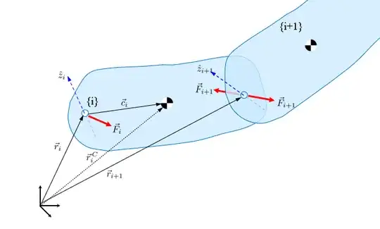
Now, consider the free body diagram above for body i and that the constraint forces $\vec{F}_{i+1}$ from the next body are applied in equal and opposite measure to the body due to Newton's 3rd law.
Let's sum up the forces and torques of body i using the pivot location $\vec{r}_i$ as the reference point.
$$ \sum_i \vec{F} = \vec{F}_i - \vec{F}_{i+1} + m_{i}\vec{g} \tag{5} $$
where $\vec{g}$ is the gravity vector, and $m_i$ is the mass of body i
and
$$ \sum_i \vec{n} = \vec{n}_i - \left( \vec{n}_{i+1} + (\vec{r}_{i+1}-\vec{r}_i) \times \vec{F}_{i+1} \right) + \vec{c}_i \times m_{i}\vec{g} \tag{6} $$
where $\vec{c}_i$ is the location of the center of mass relative to the pivot.
Now consider the Netwon-Euler equations of motion at the center of mass $$\sum_{i}\vec{F}=m\dot{\vec{v}}^{C}_{i} \tag{7}$$ and $$\sum_{i}\vec{n}^{C}=\mathcal{I}_{i}\dot{\vec{\omega}}_{i}+\vec{\omega}_{i}\times\mathcal{I}_{i}\vec{\omega}_{i} \tag{8}$$ where $\mathcal{I}_i$ is the mass moment of inetia tensor of body i about its center of mass and along the inertial basis vectors.
To combine the two sets of two equations above we need the acceleration vector transformation $\dot{\vec{v}}_{i}^{C}=\dot{\vec{v}}_{i}+\dot{\vec{\omega}}\times\vec{c}_{i}+\vec{\omega}\times\left(\vec{\omega}\times\vec{c}_{i}\right)$ and the torque vector transformation $\sum_{i}\vec{n}=\sum_{i}\vec{n}^{C}+\vec{c}_{i}\times\sum_{i}\vec{F}$ and this results in the vector equations of dymamics
$$\small \begin{aligned}\vec{F}_{i}-\vec{F}_{i+1} + m_{i}\vec{g} & =m\left(\dot{\vec{v}}_{i}+\dot{\vec{\omega}}\times\vec{c}_{i}+\vec{\omega}\times\left(\vec{\omega}\times\vec{c}_{i}\right)\right)\\
\hline \vec{n}_{i}-\left(\vec{n}_{i+1}+(\vec{r}_{i+1}-\vec{r}_{i})\times\vec{F}_{i+1}\right) + \vec{c}_{i}\times m_{i}\vec{g} & =\mathcal{I}_{i}\dot{\vec{\omega}}_{i}+\vec{\omega}_{i}\times\mathcal{I}_{i}\vec{\omega}_{i}+\vec{c}_{i}\times\left(\vec{F}_{i}-\vec{F}_{i+1}\right)
\end{aligned} \tag{9}$$
The screw version of the above uses the location of the center of mass $\vec{r}_i^C = \vec{r}_i + \vec{c}_i$ in the following equation
$$\boxed{\boldsymbol{f}_{i} - \boldsymbol{f}_{i+1} + \boldsymbol{w}_{i} = {\bf I}_{i}\boldsymbol{a}_{i}+\boldsymbol{v}_{i}\times{\bf I}_{i}\boldsymbol{v}_{i}} \tag{DYN}$$
where
Force wrench from pivot i $$\boldsymbol{f}_{i}=\begin{Bmatrix}\vec{F}_{i}\\
\vec{n}_{i}+\vec{r}_{i}\times\vec{F}_{i}
\end{Bmatrix}$$
Force wrench from next pivot i+1 $$\begin{Bmatrix}\vec{F}_{i+1}\\
\vec{n}_{i+1}+\vec{r}_{i+1}\times\vec{F}_{i+1}
\end{Bmatrix}$$
Weight wrench of body $$\boldsymbol{w}_{i}=\begin{Bmatrix}m_{i}\vec{g}\\
\vec{r}_{i}^{C}\times m_{i}\vec{g}
\end{Bmatrix}$$
Acceleration twist of body $$\boldsymbol{a}_{i}=\begin{Bmatrix}\dot{\vec{v}}_{i}+\vec{r}_{i}\times\vec{\alpha}_{i}+\vec{v}_{i}\times\vec{\omega}_{i}\\
\dot{\vec{\omega}}_{i}
\end{Bmatrix}$$
Spatial Inertia Matrix $${\bf I}_{i}=\begin{bmatrix}m_{i} & \text{-}m_{i}\vec{r}_{i}^{C}\times\\
m_{i}\vec{r}_{i}^{C}\times & \mathcal{I}_{i}-m_{i}\vec{r}_{i}^{C}\times\vec{r}_{i}^{C}\times
\end{bmatrix}$$
Wrench Cross Product Matrix $$\boldsymbol{v}_{i}\times=\begin{bmatrix}\vec{\omega}_{i}\times\\
\left(\vec{v}_{i}+\vec{r}_{i}\times\vec{\omega}_{i}\right)\times & \vec{\omega}_{i}\times
\end{bmatrix}$$
The new concept here is that of the 6×6 spatial inertia matrix ${\bf I}_i$ which is actually factored from the screw momentum equations
$$ \underbrace{\begin{Bmatrix}\vec{p}_{i}\\
\vec{L}_{i}^{C}+\vec{r}_{i}^{C}\times\vec{p}_{i}
\end{Bmatrix}}_{\text{momentum wrench}}=\underbrace{\begin{bmatrix}m_{i} & \text{-}m_{i}\vec{r}_{i}^{C}\times\\
m_{i}\vec{r}_{i}^{C}\times & \mathcal{I}_{i}-m_{i}\vec{r}_{i}^{C}\times\vec{r}_{i}^{C}\times
\end{bmatrix}}_{\text{spatial inertia matrix}}\underbrace{\begin{Bmatrix}\vec{v}_{i}^{C}+\vec{r}_{i}^{C}\times\vec{\omega}_{i}\\
\vec{\omega}_{i}
\end{Bmatrix}}_{\text{motion twist}} \tag{10}$$
which when expandedd out results in the familiar $\vec{p}_i = m_i \vec{v}_i^C$ and $\vec{L}_i^C = \mathcal{I}_i \vec{\omega}_i$. I leave this fun exercise to the reader.
Joint Condition
If the joint provides a torque with magnitude $\Gamma_i$, then the (scalar) power through the joint is $$\mathcal{P} = \Gamma_i\, \dot{\theta}_i \tag{11}$$
In terms of screws power is defined using the inner product of the relative velocity twist $\boldsymbol{s}_i \dot{\theta}_i$ and the joint constraint wrench $\boldsymbol{f}_i$
$$\begin{aligned}\mathcal{P}= & \left(\boldsymbol{v}_{i}-\boldsymbol{v}_{i-1}\right)^{\intercal}\boldsymbol{f}_{i}\\
& =\left(\boldsymbol{s}_{i}\dot{\theta}_{i}\right)^{\intercal}\boldsymbol{f}_{i}\\
& =\left(\boldsymbol{s}_{i}^{\intercal}\boldsymbol{f}_{i}\right)\dot{\theta}_{i}
\end{aligned} \tag{12}$$
and since (11) equals (12) then we have the joint condition equation $$ \boxed{ \Gamma_{i} =\boldsymbol{s}_{i}^{\intercal}\boldsymbol{f}_{i} } \tag{JC}$$
We expand the above into the vector form to get equation S16 from the posting, given that the joint torque is zero here $\Gamma_{i} =0$
$$ \require{cancel} \begin{aligned}\Gamma_{i} & =\boldsymbol{s}_{i}^{\intercal}\boldsymbol{f}_{i}\\
& =\begin{Bmatrix}\vec{r}_{i}\times\hat{z}_{i}\\
\hat{z}_{i}
\end{Bmatrix}^{\intercal}\begin{Bmatrix}\vec{F}_{i}\\
\vec{n}_{i}+\vec{r}_{i}\times\vec{F}_{i}
\end{Bmatrix}\\
& =\left(\vec{r}_{i}\times\hat{z}_{i}\right)\cdot\vec{F}_{i}+\hat{z}_{i}\cdot\left(\vec{n}_{i}+\vec{r}_{i}\times\vec{F}_{i}\right)\\
& =\hat{z}_{i}\cdot\vec{n}_{i}+\cancel{\left(\vec{r}_{i}\times\hat{z}_{i}\right)\cdot\vec{F}_{i}+\hat{z}_{i}\cdot\left(\vec{r}_{i}\times\vec{F}_{i}\right)}\\
\Gamma_{i} & =\hat{z}_{i}\cdot\vec{n}_{i}
\end{aligned} \tag{13}$$
System of two freely floating connected bodies
Working out the equations of two connected bodies
$$\begin{aligned}\text{velocity kinematics [VK]} & & \boldsymbol{v}_{2}-\boldsymbol{v}_{1} & =\boldsymbol{s}_{2}\dot{\theta}_{2}\\
\hline \text{acceleration kinematics [AK]} & & \boldsymbol{a}_{2}-\boldsymbol{a}_{1} & =\boldsymbol{s}_{2}\ddot{\theta}_{2}+\boldsymbol{v}_{2}\times\boldsymbol{s}_{2}\dot{\theta}_{2}\\
\text{rigid body dynamics [DYN]} & & -\boldsymbol{f}_{2}+\boldsymbol{w}_{1} & ={\bf I}_{1}\boldsymbol{a}_{1}+\boldsymbol{v}_{1}\times{\bf I}_{1}\boldsymbol{v}_{1}\\
\text{rigid body dynamics [DYN]} & & \boldsymbol{f}_{2}+\boldsymbol{w}_{2} & ={\bf I}_{2}\boldsymbol{a}_{2}+\boldsymbol{v}_{2}\times{\bf I}_{2}\boldsymbol{v}_{2}\\
\text{joint condition [JC]} & & \boldsymbol{s}_{2}^{\intercal}\boldsymbol{f}_{2} & =0
\end{aligned}$$
Counting up the equations and excluding the first one (vector kinematics) since velocities are considered known when solving dynamics, we have three spatial equations = 6 vector equations = 18 component equations plus the last equation, which is a scalar equation for a total of 19 component equations. We also have the following unknowns $\boldsymbol{a}_1$, $\boldsymbol{a}_2$, $\boldsymbol{f}_2$, and $\ddot{\theta}_i$ which are 6 vector quantities plus one scalar exactly 19 unknown components and thus we have a 19×19 system of equations to solve.
References


