Formulating the catenary problem as a variational problem

Question

I am interested in studying the curve a string follows when fixed by two points and subject to a (uniform) gravitational field. Say the string has a constant length $L$ and is fixed on two points A, B such that they have height $y=0$, thus taking at said height the origin of gravitational potential energy. I am interested in obtaining the curve (in natural parameter) $\vec x (s)=(x(s), y(s))$ the string follows.

The energy differential on point $s$ of the parametrization shall be:

$$dE(s)=dm g y(s)=\rho g y(s)ds$$

And integrating over all the curve, we get:

$$E=\rho g\int_0^Ly(s)ds$$

Intuitively, the curve followed by the string shall be such that the energy is minimal, and so I want to minimize the string's energy subject to the constraint:

$$\dot x^2+\dot y^2=1$$

I have tried to introduce this constraint on the energy integral with a Lagrange multiplier like so:

$$S=\int_0^L(\rho g y-\lambda(\dot x^2+\dot y^2-1))ds$$

where I have defined my analogue of "action", and so the Lagrangian of the system shall be the integrand. Now I apply the Euler-Lagrange equations:

$$\frac{\partial \mathcal L}{\partial x}-\frac{d}{ds}\frac{\partial \mathcal L}{\partial \dot x}=0$$

$$\frac{\partial \mathcal L}{\partial y}-\frac{d}{ds}\frac{\partial \mathcal L}{\partial \dot y}=0$$

and obtain the following 2-ODE system:

$$\lambda \dot x=\text{constant}$$ $$\frac{d}{ds}(\lambda \dot y)=\frac{1}{2}\rho g$$

but solving them gives me a parabola, not a hyperbolic cosine as I was expecting. What is it that I'm not seeing?

Answer 1

You need a separate Lagrange multiplier for each point on the string. So the quantity to be minimised is $$ E= \int_0^L \left\{ \rho gy(s)+ \lambda(s)\left (\frac12 \dot x^2+\frac 12 \dot y^2\right)\right\}ds,. $$ where $s$ is the arc-length. Then the EL equations are $$ 0= -\frac{d}{ds}(\lambda(s) \dot x(s))\\ 0=\rho g- \frac{d}{ds}(\lambda(s) \dot y(s)), $$ which, after multiplication by $\delta(s)$ give the equilibrium of the a small segement of string of length $\delta s$ at $s$. The constraint $\dot x^2+\dot y^2=1$ allows is to set $\dot x= \cos\theta$ and $\dot y=\sin\theta$. Comparing with the horizontal and vertical force balance equations on the string segment $$ 0= -\frac{d}{ds}(T(s) \cos \theta),\\ 0=\rho g- \frac{d}{ds}(T(s) \sin\theta (s)), $$ we see that $\lambda(s)=T(s) $ is the tension in the string at the point $s$.

Answer 2

The problem is actually less hard to solve when first solving for any length $L$, and only after that general problem is solved narrow down to a specific length of the string.

The reason why that is possible is interesting, so I will take the space to discuss that.

For simplicity we position the two suspension points at the same height.

with:
$s$ separation between suspension points
$L$ length of the string.

There is a scale invariance.
For a given ratio $L$/$s$ the shape of the suspended string is the same.

So if you have a setup, and you lengthen the string the suspended string sags. Then a subsection of the sagged string that has the same $L$/$s$ ratio has the same shape as the string before the lengthening.

It follows that a single solution will fit all cases; to fit a specific case; it is a subsection of the total curve such that it has $L$/$s$ in the ratio that you need.

As we know: to find the point in variation space such that the integral of the potential energy is minimal we identify a point in variation space such that the derivative of the potential energy integral is zero.

With:
$x$ horizontal coordinate
$y$ vertical coordinate

The integration will be with respect to the horizontal coordinate. The integration consists of each element of the string corresponding to the length $dx$.

For simplicity I set the (gravitational) acceleration to 1, and I set the density of the string (per unit of length) to 1

Here is the integral that we need to differentiate with respect to variation:

$$ \int_0^x y \ \sqrt{1 + (y')^2} \ dx \tag{1} $$

About that Lagrangian for this case:

$$ y \ \sqrt{1 + (y')^2} \tag{2} $$

For each subsection $dL$ along the length of the string we evaluate the contribution to the total potential energy.

To make the problem tractable we need to restate the contribution from $dL$ in terms of $x$ and $y$.

$$ (dL)^2=(dx)^2+(dy)^2 \quad \Leftrightarrow \quad \frac{dL}{dx} = \sqrt{1 + \left(\frac{dy}{dx}\right)^2} $$

From ($x$) to ($x+dx$) the contribution to the potential energy is proportional to:
-the height, which here is the y-coordinate
-the ratio of string length to the length $dx$, which is the ratio $\tfrac{dL}{dx}$

Directly inserting the Lagrangian (2) into the Euler-Lagrange equation gives a gnarly expression, but fortunately there is another way.

In that Lagrangian (2) there is no factor with the x-coordinate directly. That's because the thing that causes the shape to form, gravity, is a function of the y-coordinate only.

That not-dependent-on-the-x-coordinate-directly property allows a form of the Euler-Lagrange equation with a differentiation with respect to x backed out.

On mathematics stackexchange there is an answer by me to a question titled: The relation between the Euler-Lagrange equation and the Beltrami identity

(That question had been submitted by me, and a comment to the question allowed me to see what had eluded me.)

The Beltrami identity:

$$ F - y' \frac{\partial F}{\partial y'} = C \tag{3} $$

Substitute $F$ in the Beltrami identity with the Lagrangian.
The expression looks difficult but many of the terms drop away against each other:

$$ y \ \sqrt{1 + y'^2} - \frac{y \ y'^2}{\sqrt{1 + y'^2}} = \frac{y \big((1 + y'^2) -y'^2 \big)}{\sqrt{1 + y'^2}} = \frac{y}{\sqrt{1 + y'^2}} \tag{4} $$

Set the condition that (4) must be a constant:

$$ \frac{y}{\sqrt{1 + y'^2}} = C \qquad \Leftrightarrow \qquad \frac{y}{C} = \sqrt{1 + y'^2} \tag{5} $$

For now I simplify by setting the value of the constant $C$ to 1.

(Thanks to Daniel Rubin for pointing out the following strategy to solve (5): the Catenary (Youtube video))

Square both sides. Squaring both sides introduces an extraneous solution, so at a later stage we must discard that.

$$ y^2 = 1 + \left(\frac{dy}{dx}\right)^2 \tag{6} $$

Take the derivative with respect to $x$:

$$ 2y\frac{dy}{dx} = 2 \frac{dy}{dx} \frac{d^2y}{dx^2} \tag{7} $$

divide by $2\tfrac{dy}{dx}$:

$$ y = \frac{d^2y}{dx^2} \tag{8} $$

(8) informs us that the function that solves the problem has the property that when you differentiate it twice you are back to the same function.

Two functions satisfy (8): the hyperbolic sine and the hyperbolic cosine. Of the two the hyperbolic cosine satisfies (5).

With the problem now solved for any ratio of $L$/$s$:
Work out which subsection of the hyperbolic cosine satisfies the fixed length $L$ of the string.

Answer 3

1. The extended Lagrangian $L$ uses the arc-length $s$ as an independent variable$^1$ $$\begin{align} L[x,y,\lambda]~=~&\int_0^{\ell} \!ds~{\cal L}(x,y,\lambda,x^{\prime},y^{\prime}), \cr {\cal L}(x,y,\lambda,x^{\prime},y^{\prime}) ~=~&\frac{\lambda}{2}(x^{\prime 2}+y^{\prime 2}-1)-{\cal V}(y),\cr {\cal V}(y)~=~&\rho g y,\end{align}\tag{1} $$ where the extended Lagrangian density ${\cal L}$ is a Lagrange multiplier $\lambda(s)$ times a constraint minus the potential energy density ${\cal V}$.

2. We impose Dirichlet boundary conditions $$ \begin{align} x(s\!=\!0)~=~&x_A, \qquad x(s\!=\!\ell)~=~x_B,\cr y(s\!=\!0)~=~&y_A, \qquad y(s\!=\!\ell)~=~y_B, \tag{2} \end{align} $$

3. The $x$ variable is a cyclic variable, so the $x$-momentum $$p_x~=~\frac{\partial{\cal L}}{\partial x^{\prime}}~=~\lambda x^{\prime}\tag{3}$$ is a COM.

4. Let's consider the Routhian density, $$ {\cal R}(y,\lambda,y^{\prime})~=~x^{\prime}p_x-{\cal L}~\stackrel{(1)+(3)}{=}~\frac{\lambda}{2}(1-y^{\prime 2})+\frac{p_x^2}{2\lambda}+{\cal V},\tag{4}$$ cf. e.g. my Phys.SE answer here.

5. The EL equation for the Lagrange multiplier is $$\lambda~\stackrel{(4)}{=}~\pm\frac{p_x}{\sqrt{1-y^{\prime 2}}}.\tag{5}$$

6. Integrating out/eliminating the Lagrange multiplier $\lambda$ produces a square root Routhian density: $$ {\cal R}_0(y,y^{\prime})~\stackrel{(4)+(5)}{=}~ \pm p_x\sqrt{1-y^{\prime 2}}+{\cal V}. \tag{6}$$

7. The $y$-momentum is $$ p_y~=~-\frac{\partial {\cal R}_0}{\partial y^{\prime}}~=~\pm p_x\frac{y^{\prime}}{\sqrt{1-y^{\prime 2}}}.\tag{7} $$

8. The energy density $${\cal E}~=~y^{\prime}p_y+{\cal R}_0~\stackrel{(6)+(7)}{=}~ \pm \frac{p_x}{\sqrt{1-y^{\prime 2}}}+{\cal V}\tag{8} $$ is conserved along $s$ because of no explicit $s$-dependence.

9. By shifting the $y$-coordinate we may assume that ${\cal E}=0$. Solving the ODE (8) leads to $$ \sqrt{y^2-a^2}~=~s-s_0, \qquad a~:=~\mp\frac{p_x}{\rho g}.\tag{9} $$

10. We may assume that $s_0=0$. So $$\begin{align} y~\stackrel{(9)}{=}~&\pm\sqrt{s^2+a^2}\cr\Downarrow~&\cr \dot{y}~=~&\pm\frac{s}{\sqrt{s^2+a^2}}\cr\Downarrow~&\cr \dot{x}~=~&\pm\frac{a}{\sqrt{s^2+a^2}}\cr\Downarrow~&\cr \frac{dy}{dx}~=~&\frac{y^{\prime}}{x^{\prime}}~=~\pm\frac{s}{a}~\stackrel{(9)}{=}~\pm\frac{\sqrt{y^2-a^2}}{a},\end{align}\tag{10} $$ which is known to lead to the catenary.

---

$^1$ There is no kinetic energy since it is a static problem. A prime denotes differentiation wrt. the arc-length $s$. Concerning the status of the constraint, i.e. holonomic vs. non-holonomic, see also e.g. this related Phys.SE post.

Answer 4

In this answer the catenary problem is solved with differential calculus.

The fact that the catenary problem can be solved both with differential calculus and with variational calculus is very, very significant. It is an instance of a general property of application of calculus of variations in physics.

Differential calculus and variational calculus are closely related.
Note that the Euler-Lagrange equation is a differential equation. There is a reason that the Euler-Lagrange equation is a differential equation.

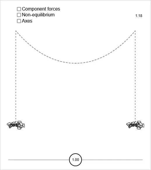
The image shows a hanging chain in a state of force equilibrium.

The image is stylized, the idea is that at the cusps the chain can move freely. Imagine there are frictionless rollers at the cusps.
The length of the vertical sections is set up to provide the amount of tension force that is required for force equilibrium with the length of chain hanging between the cusps.

(The image is a screenshot of an interactive diagram that is on my own website.)

First:
To set up the differential equation for the shape of the catenary.

Since the shape is symmetric it is sufficient to evaluate from the midpoint to the cusp.

The catenary is in force equilibrium at every point along its length.
In particular: there is no bending force anywhere along the length. (If there would be a bending force then the string would move in that direction, but the string isn't moving.) It follows: at every point along the length of the string the local tension force is tangent to the local slope.

With:
$T_H$ The horizontal component of the tension
$λ$ The weight per unit of length
$L$ the length of the chain from the midpoint to the x-coordinate.

The weight that has to be supported at coordinate $x$ is given by multiplying the length $L$ with the weight per unit of length: $λL$

The differential equation setup here uses the following property: gravity is acting in the vertical direction, therefore there is no gradient in the horizontal component of the tension. That is: the horizontal component of the tension is not a function of the x-coordinate, but constant.

In preparation: from midpoint to cusp the slope of the curve increases; the length of chain per unit of x-coordinate increases accordingly. (1) gives an expression for dL/dx, which will later be used.

$$ (dL)^2=(dx)^2+(dy)^2 \quad \Leftrightarrow \quad \frac{dL}{dx} = \sqrt{1 + \left(\frac{dy}{dx}\right)^2} \tag{1} $$

At every point along the catenary the slope of the curve is equal to the ratio of horizontal tension component and vertical tension component:

$$ \frac{dy}{dx} = \frac{\lambda L}{T_H} \tag{2} $$

We need an expression with the derivative of $L$ with respect to $x$, so that (1) can be put to use. $T_H$ and $λ$ are constants, so we can treat $λ$/$T_H$ as a constant multiplication factor.

$$ \frac{dy}{dx} = L \frac{\lambda}{T_H} \tag{3} $$

Taking the derivative:

$$ \frac{d^2y}{dx^2} = \frac{\lambda}{T_H} \frac{dL}{dx} \tag{4} $$

Combining (4) and (1) allows us to eliminate the quantity $dL$, arriving at a differential equation that is is purely in terms of the cartesian coordinates $x$ and $y$:

$$ \frac{T_H}{\lambda}\frac{d^2y}{dx^2} = \sqrt{1 + \left(\frac{dy}{dx}\right)^2} \tag{5} $$

To simplify the quantity $T_H/\lambda$ is set so a value of 1, so that it can be omitted. (We have the option of putting it back later.)

$$ \frac{d^2y}{dx^2} = \sqrt{1 + \left(\frac{dy}{dx}\right)^2} \tag{6} $$

At this point we have with (6) reached an equation that is very similar to equation (6) of my earlier answer to this question, in which the problem was solved with calculus of variations.

We make the substitution $\tfrac{dy}{dx}=u$, and we square both sides. Squaring both sides introduces an extraneous solution, so at a later stage we must discard that.

$$ \left(\frac{du}{dx}\right)^2 = 1 + u^2 \tag{7} $$

Differentiating with respect to $x$ allows the expression to be simplified:

$$ 2\frac{du}{dx}\frac{d^2u}{dx^2} = 2u\frac{du}{dx} \tag{8} $$

After dividing by $2\tfrac{du}{dx}$:

$$ \frac{d^2u}{dx^2} = u \tag{9} $$

So the solution to the equation is a function with the property that if you differentiate it twice you are back to the original function. That narrows the options down to the hyperbolic sine and the hyperbolic cosine. Checking against the original equation rules out the hyperbolic sine.

(10) incorporates the ratio $\tfrac{T_H}{λ}$ such that it satisfies (5)

$$ y = \tfrac{T_H}{\lambda} \cosh \left(\tfrac{\lambda}{T_H} x \right) \tag{10} $$

Comparison with application of calculus of variations

There are striking parallels between the differential approach and the variational approach.

The differential approach capitalizes on the fact that the horizontal tension component is not a function of the x-coordinate.
In effect the variational approach capitalizes on the same property. Since the Lagrangian is not explicitly a function of the x-coordinate the Beltrami identity can be used.

The catenary problem is by nature a force equilibrium problem. The solution is a curve such that at every point along the curve the forces are in equilbrium.

The variational approach takes as input an expression for the total potential energy. As we know: potential energy is defined as the negative of work done: From an initial height $y_i$ to a final height $y_f$:

$$ E_p = - \int_{y_i}^{y_f} F \ dy \tag{11} $$

For the catenary problem it is sufficient to sweep out variation in one direction only: the direction of gravity. That is the vertical direction, the direction of the y-axis

Note especially:
The Euler-Lagrange equation takes the derivative in the direction of the variation of the variational equation.

That means:
The strategy of the variational approach to solving the catenary problem consists of differentiating the potential energy with respect to the vertical position coordinate.

That is to say:
The variational approach to solving the catenary problem consists of transforming the variational expression to the corresponding force equilibrium expression.

Discussion

As we know: whereas for many types of equation the solution is a value, the solution to a differential equation is a function. The solution space of a differential equation is a space of functions.

That is enforced by the demand that the differential relation stated in the equation must be satisfied for all parts of the curve concurrently. In that sense a differential equation is intrinsically a global equation; it is to be satisfied everywhere concurrently.

A variational equation has that property too: the solution to a variational equation is a function. The solution space of a variational equation is a space of functions.

The catenary problem has the following property:
Every subsection of the catenary problem is itself an instance of the catenary problem. We can divide in subsections, and solve down at subsection level. In effect the solutions at subsection level are concatenated to the overall solution. (In a numerical analysis implementation of variational approach that type of subdivision is used.) There is no limit to the level of subdivision; the divisibility in subsections extends all the way to infinitesimally small subsections.

I will refer to that property of a problem as being concatenable.

By contrast, take the traveling salesman problem
That problem is not concatenable.
A solution for a subsection of the set of nodes is highly unliky to be part of the solution for an expanded set of nodes.

In order for a problem to yield to variational approach the problem must be concatenable.

Answer 5

Euler--Lagrange Equation and Solution

We consider the functional $$ \mathcal{L} = y \sqrt{1 + (y')^2} $$

The Euler--Lagrange equation is given by: $$ \frac{d}{dx} \left( \frac{\partial \mathcal{L}}{\partial y'} \right) - \frac{\partial \mathcal{L}}{\partial y} = 0 $$

We compute the partial derivatives: \begin{align*} \frac{\partial \mathcal{L}}{\partial y} &= \sqrt{1 + (y')^2}, \\ \frac{\partial \mathcal{L}}{\partial y'} &= \frac{y y'}{\sqrt{1 + (y')^2}} \end{align*}

Taking the total derivative: $$ \frac{d}{dx} \left( \frac{y y'}{\sqrt{1 + (y')^2}} \right) = \frac{(y')^2}{\sqrt{1 + (y')^2}} + y \cdot \frac{y''}{(1 + (y')^2)^{3/2}} $$

Substitute into the Euler--Lagrange equation: \begin{align*} \frac{(y')^2}{\sqrt{1 + (y')^2}} + y \cdot \frac{y''}{(1 + (y')^2)^{3/2}} - \sqrt{1 + (y')^2} &= 0 \\ \Rightarrow \quad \frac{y y'' - (y')^2 - 1}{\left(1 + (y')^2\right)^{3/2}} &= 0 \end{align*}

Multiply both sides by $\left(1 + (y')^2\right)^{3/2}$: $$ y y'' = (y')^2 + 1 \quad \Rightarrow \quad y'' - \frac{(y')^2 + 1}{y}=0 $$

Solution

The general solution to this differential equation with the initial conditions $~y(0)=y_0~,\dot y(0)=0 $ is: $$ \boxed{y(x) = y_0 \cosh\left( \frac{x}{y_0} \right)} $$

This is the classic catenary curve, which describes the shape of a hanging flexible chain or cable under uniform gravity. Beautiful connection between calculus of variations and physics!

---

---

consider your functional $$\mathcal{L}=\rho\,g\,y(s)+\frac 12 \lambda(s)\,(x'^2+y'^2)$$

with EL we obtain: \begin{align*} &\,\lambda\,{\it x''}+\,\lambda' \,{\it x'}=0\\ &\,\lambda\,{\it y''}-\rho\,g+\,\lambda' \,{\it y'}=0 \end{align*} and from the constraint equation $e_c=~x'^2+y'^2=1 ~$ \begin{align*} & e_c''=x'\,x''+y'\,y=0 \end{align*}

solving these 3 equations for $~x``~,y''~,\lambda'~$

\begin{align} & x''=-\rho\,g\,\frac{x'\,y'}{\lambda}\quad\quad &(1)\\ &y''=\rho\,g\,\frac{x'^2}{\lambda}\quad\quad &(2)\\ &\lambda'=\rho\,g\,y'\quad\quad &(3) \end{align}

Analytical Solution

with Eq. (3) \begin{align*} \lambda=\rho\,g\,\int dy=\rho\,g\,y+c\quad \text{with}\quad\lambda(0)=0\quad\Rightarrow c=0 \end{align*} thus Eq. (1) ,(2)

\begin{align} & x''=-\rho\,g\,\frac{x'\,y'}{\rho\,g\,y}\\ &y''=\rho\,g\,\frac{x'^2}{\rho\,g\,y} \end{align}

Given the constraint: $$ \left( \frac{dx}{ds} \right)^2 + \left( \frac{dy}{ds} \right)^2 = 1 $$ and the governing equations, the analytical solution is given by:

$$ \begin{aligned} y(s) &= y_0 \cosh\left( \frac{x(s)}{y_0} \right), \text{Ansatz}\quad\Rightarrow\\ x(s) &= y_0 \sinh^{-1}\left( \frac{s}{y_0} \right). \end{aligned} $$

Equivalently, solving for $y(s)$ in terms of $s$:

$$ y(s) = y_0 \cosh\left( \sinh^{-1}\left( \frac{s}{y_0} \right) \right) = \sqrt{s^2 + y_0^2} $$