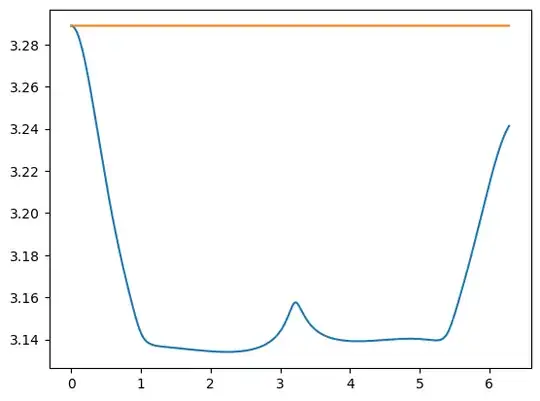
Numerical Solution of the circular restricted three body problem

Question

I am trying to numerically solve the differential equations in the planar circular restricted three-body problem. In the rotating frame, the differential equations are given by \begin{equation} \begin{split} \ddot{x}&=2\dot{y}+x-\frac{(1-\mu)(x+\mu)}{s_1^3}-\frac{\mu(x-1+\mu)}{s_2^3} \\ \ddot{y}&=-2\dot{x}+y-\frac{(1-\mu)y}{s_1^3}-\frac{\mu y}{s_2^3} \end{split} \end{equation} where the non-dimensional distances are given by \begin{equation} s_1=\sqrt{(x'+\mu)^2+(y')^2+(z')^2} \qquad \text{and} \qquad s_2=\sqrt{(x'-1+\mu)^2+(y')^2+(z')^2} \end{equation} I have converted this to a set of ODE's and I am using scipys solve_ivp, here is the code

mu = 1.2151e-2
def dSdt(t, S):
    x, v_x, y, v_y = S
    return [
        v_x,
        2 * v_y
        + x
        - ((1 - mu) * (x + mu)) / ((np.sqrt((x + mu)**2 + y**2))**3)
        + (mu * (x - 1 + mu)) / ((np.sqrt((x - 1 + mu)**2 + y**2))**3),
        v_y,
        -2 * v_x
        + y
        - ((1 - mu) * y) / ((np.sqrt((x + mu)**2 + y**2))**3)
        - (mu * y) / ((np.sqrt((x - 1 + mu)**2 + y**2))**3),
    ]
x_0 = 0.8372 - 0.1
v_x0 = 0
y_0 = 0
v_y0 = 0
S_0 = (x_0, v_x0, y_0, v_y0)
t = np.arange(0, 2np.pi, 0.001)
sol = solve_ivp(dSdt, (0, 2np.pi), y0=S_0, method='DOP853', t_eval=t, rtol=1e-13, atol=1e-14)

However, I am not very confident in the subsequent plots and when i compute the Jacobi constant (constant of motion in the problem) given by $$ C=-(\dot{x}^2+\dot{y}^2+\dot{z}^2)-2\tilde{U} $$ where $\tilde{U}$ is the effective potential $$ \tilde{U}=-\frac{1}{2}(x^2+y^2)-\frac{(1-\mu)}{s_1}-\frac{\mu}{s_2}-\frac{1}{2}(1-\mu)\mu $$ I get a standard deviation of $0.038$ over a single period of the primaries which is orders of magnitude higher than the specified tolerance. The plot below shows the discrepancy:
I am unsure as to how I can get rid of this error and I don't really feel that I can trust the plots I get when it seems to be inaccurate. I have tried using the different schemes provided by solve_ivp, changing the tolerance and step sizes but nothing seems to help. It also seems very odd that I am getting such a large error as the code I am using is very similar to what this guy does in this YouTube video: https://www.youtube.com/watch?v=WeXEPHzJqQQ&list=PLUeHTafWecAXDF9vWi7PuE2ZQQ2hXyYt_&index=11 around the 36 minute mark. He doesn't get anywhere close to the error that I am getting. Here is the code for determining the Jacobi integral:

def jacobi_integral(position, velocity):
    s_1 = np.sqrt((position[:,0]+mu)**2+(position[:,1])**2)
    s_2 = np.sqrt((position[:,0]-1+mu)**2+(position[:,1])**2)
effective_potential = (-1/2)*((position[:,0]**2+position[:,1]**2))-(1-mu)/s_1-mu/s_2-((1-mu)*mu)/2

jacobi_constant = -((velocity[:,0])**2+(velocity[:,1])**2)-2*effective_potential

return jacobi_constant

I have looked into symplectic integration schemes, but they don't seem applicable from my limited understanding since I have velocity-dependent terms in my differential equations. If anyone has any tips or suggested solutions, I would greatly appreciate any input!

Numerical Solution of the circular restricted three body problem

0 Answers0