Gauss law for surface charge distributions

Question

I have read that the Maxwell's equations summarize the entire classical electrodynamics, but while studying electrostatics I encountered the gauss's law for electric fields fails when the imaginary closed surface coincides with the charged surface. For example, if we want to calculate the electric field of a charged sphere with uniform surface charge density $\sigma$ on the surface of the sphere, we face that there is a discontinuity in the electric field. This discontinuity cannot be observed by using Gauss's law for electric fields. Thus, I observed that I can't apply Gauss law here and have to resort to Coulomb's law (I am considering the sphere to be at rest in an inertial frame). So, am I wrong in saying that Maxwell's equations are not complete. Is there any way of summarizing classical electrodynamics without encountering such exceptions where the laws do not hold?

Here, as I am unable to solve it using Gauss's law, I solved using Coulomb's law and here is the proof.

As coulomb's law (here we can apply Coulomb's law because this is an electrostatics problem) is only valid for a point charge, I consider a tiny square element (it approaches a point as limit of its dimensions tends to 0). To find the area of this tiny area element I parameterized the spherical surface as: $\vec r = (R\cos(\theta), R\sin(\theta)\sin(\phi), R\sin(\theta)\cos(\phi))$. Here $\theta$ is the angle made by the vector and x-axis while $\phi$ is the angle made by the projection of the vector in y-z plane with the z-axis. So, $\theta \in [0, \pi]$ and $\phi \in [0, 2\pi)$. Then, we can say that

$$dA=\left|\frac{\partial \vec r}{\partial \theta} \times \frac{\partial \vec r}{\partial \phi}\right|d\theta d\phi=R^2 \sin(\theta) d\theta d\phi$$

After applying the limits mentioned above and performing the following integral,

$$\vec E = \iint \frac{k(\sigma\cdot dA) \vec r}{|\vec r|^3} = \frac{\sigma}{2\epsilon_0} \hat r$$

Here $\sigma$ refers to the surface charge density of the sphere.

Answer 1

Before providing possible approaches:

• Maxwell equations, along with Lorentz force, are the governing equations of classical electromagnetism (treating irregularities as described below);
• Coulomb force directly comes from the combined application of Lorenz force (in steady condition) and Gauss's law for the electric field, when you deal with point charges. It adds nothing to Maxwell equations, and it's a direct consequence.

The differential/local form of Maxwell equations only hold if the fields are "regular enough", being a set of differential equations. If you want/need to use differential form of the equations, I'd try two approaches:

Approach 1. You could "make them work" using generalized functions, like Dirac's delta and steps to treat point charges, surface charges,...

Approach 2. You could 1. partition the domain in a set of regions where the fields are "regular enough"; 2. connect these regions with boundary/jump conditions across the manifolds where "irregularities" arise

Global/integral form of the equations work seamlessly even with functions not regular enough for the differential form to hold, but they usually provide you less detailed information, if you can't exploit symmetry and apply them on particular domains that give you all the information you need. These equation, for a steady domain $V$, read

$$\begin{cases} \oint_{\partial V} \mathbf{d} \cdot \mathbf{\hat{n}} = Q^{int}_{V} \\ \oint_{\partial S} \mathbf{e} \cdot \mathbf{\hat{t}} + \frac{d}{dt} \int_{S} \mathbf{b} \cdot \mathbf{\hat{n}} = 0 \\ \oint_{\partial V} \mathbf{b} \cdot \mathbf{\hat{n}} = 0 \\ \oint_{\partial S} \mathbf{h} \cdot \mathbf{\hat{t}} - \frac{d}{dt} \int_{S} \mathbf{d} \cdot \mathbf{\hat{n}} = I_{S} \\ \end{cases}$$

being $Q^{int}_V$ the total electric charge in the volume $V$ and $I_S$ the electric current through surface $S$.

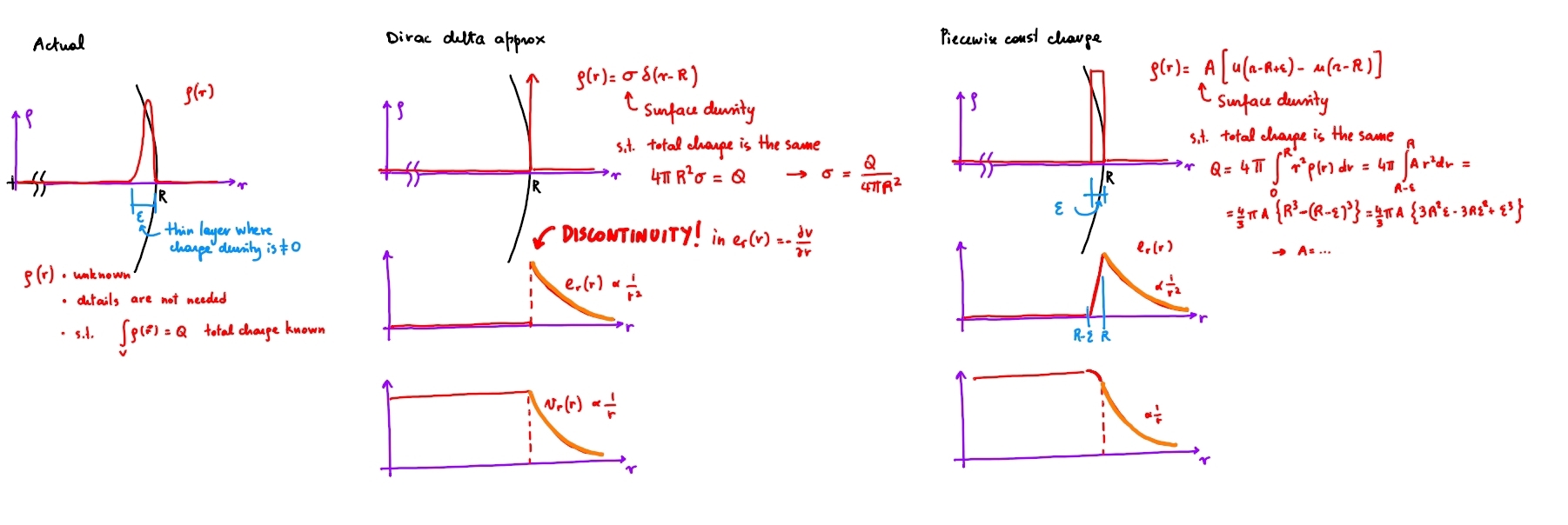
Edit. Here you can find a possible approach, using two different models of the thin distribution of electric charge (with no detail known, except for radial symmetry and total charge), one with Dirac's delta and one with uniform charge in a finite-thickness layer close to the surface of the sphere. As you can see, if you use the Dirac's delta model, the electric field is discontinuous at the surface, so it's meaningless to look for a value there (if you don't further regularize the integral of the Dirac delta, finding the average of the values on the sides of the jump); otherwise, if you use the finite approximation, the electric field is continuous and you can find a value of the electric field for each value of $r$.

Edit 2. - Evaluation of the electric field using Gauss' law and generalized function. In this paragraph, I'll show you how to use a differential equation with generalized functions, as the one required to represent a surface distribution in a 3-dimenisonal domain.

Using spherical coordinates, and the assumption of spherical symmetry, here the charge density is represented by the generalized function

$$\rho(r) = \sigma \delta(r-R) \ .$$

Gauss' law $\nabla \cdot \mathbf{e} = \frac{\rho}{\varepsilon}$ in spherical coordinates reads

$$\frac{1}{r^2} \frac{d}{d r} \left( r^2 e_r \right) = \frac{\rho}{\varepsilon} \ ,$$

and it can be recast as

$$\frac{d}{d r} \left( r^2 e_r \right) = r^2 \frac{\rho}{\varepsilon} \ .$$

Direct integration of the last equation reads

$$\begin{aligned} r^2 e(r) - r_0^2 e(r_0) & = \frac{\sigma}{\varepsilon} \int_{r_0}^{r} x^2 \delta(x - R) d \, x = \\ & = \frac{\sigma}{\varepsilon} R^2 u(r-R) \ , \end{aligned}$$

being $u(r)$ the step function

$$u(r) = \begin{cases} 0 & , \quad r < 0 \\ 1 & , \quad r > 0\end{cases}$$

Remark. This is the discontinuous function that appears in the diagrams above, and that you can regularize. But if you use this "Dirac's delta"-approach this function is discontinuous and, as I've already mentioned, it's meaningless to look for a value in $r=R$; if you really want, you can set $\frac{1}{2}$ keeping in mind that it's just the average value of the jump.

Setting $r_0 = 0$, the analytic expression (piece-wise continuous) of the radial component of the electric field reads

$$e(r) = \frac{\sigma}{\varepsilon} \frac{R^2}{r^2} u(r-R) = \begin{cases} 0 & , \quad r < R \\ \frac{\sigma}{\varepsilon} \frac{R^2}{r^2} &, \quad r > R \ .\end{cases} $$

Answer 2

Assuming $\sigma$ as a mathematically surface charge density, and integrating for a point very close to the surface (outside or inside), the limit is $E = \frac{\sigma}{2\epsilon_0}$.

According to that "exactly zero thickness surface" approach, the field is $\frac{\sigma}{2 \epsilon_0}$ exactly at the surface. It falls sharply asymptotically to zero inside. And grows sharply outside until gets $\frac{\sigma}{\epsilon_0}$. Only then, it starts to decrease with the square of the distance.

I don't think it is right. For example, it is strange that the field outside (and very close to the surface) grows with the distance for a while before decay.

The correct procedure is to use volumetric density of charges $\rho$. In this case, the field is zero inside, grows sharply (for a thin shell) from zero to $\frac{Q}{4\pi R_e^2\epsilon_0}$ at the outside surface, and is $\frac{Q}{4\pi r^2\epsilon_0}$ outside.

As for a shell, $$\frac{Q}{4\pi R_e^2} = \rho \frac{4}{3}\frac{\pi(R_e^3 - R_i^3)}{4\pi R_e^2}$$ the field becomes at the external surface of a thin shell: $$E \approx \frac{\rho \Delta R}{\epsilon_0}$$ If we rename $\rho \Delta R = \sigma$ (surface density of charges) then the field at the external surface is:$$E \approx \frac{\sigma}{\epsilon_0}$$

All this can be obtained by using the Coulomb law, and integrating the field along the shell. The Coulomb law is the general solution for the Gauss (differential) law.

However, for a spherical symmetric case like that, it is possible to use the divergence theorem: $\int_V \nabla\cdot\vec E = \int_S \vec E\cdot\vec n dS$ because due to the symmetry, $\vec E$ is always radial and has the same magnitude for a given radius. For a point outside the sphere: $$\int_V \nabla\cdot\vec E = \frac{\rho 4\pi R^2 \Delta R}{\epsilon_0} = \frac{\sigma 4\pi R^2}{\epsilon_0} = \int_S \vec E\cdot\vec n dS = 4\pi r^2 E_r$$ $$E_r = \frac{\sigma R^2}{\epsilon_0 r^2}$$ For a point just at the surface: $$E_r = \frac{\sigma}{\epsilon_0}$$

A similar approach shows that the field is zero in the interior and grows from zero to $E_r = \frac{\sigma}{\epsilon_0}$ in the shell.

$\vec E(r)$ is a continuous function, but the gradient of the field inside the shell is sharper for thinner shells.