21

Some other physics teachers and I were discussing an AP problem about a potential experiment for measuring $g$ and disagreed on the best way to use a line of best fit to analyze the data.

The experiment measures the acceleration of an Atwood machine and uses the theoretical relation $a= \frac{m_1-m_2}{m_1+m_2}g$. The AP problem wants students take some sample data, plot $a$ versus $\frac{m_1-m_2}{m_1+m_2}$, and interpret the slope of the line as an experimental value of $g$.

The question is whether the line of best fit should be made to pass through the origin or not. That is, should we try to fit to the form $a = mz+b$ to the data or just $a=mz$. My argument is that the model we have does not have a constant term and adding one would be overfitting so we should not fit to $a = mz+b$ just like we shouldn't fit to $a = mz^2 +bz+c$. Another teacher argued that we should treat the data as the data and fit its true line of best fit, independent of what we think the model might be.

Obviously think I am right, but am I mistaken?

Qmechanic
  • 220,844

7 Answers7

38

You should almost always include the intercept. Not including the intercept can lead to bias in your estimate of the slope in your model as well as other problems.

it is generally a safe practice not to use regression-through-the origin model and instead use the intercept regression model. If the regression line does go through the origin, b0 with the intercept model will differ from 0 only by a small sampling error, and unless the sample size is very small use of the intercept regression model has no disadvantages of any consequence. If the regression line does not go through the origin, use of the intercept regression model will avoid potentially serious difficulties resulting from forcing the regression line through the origin when this is not appropriate.

(Kutner, et al. Applied Linear Statistical Models. 2005. McGraw-Hill Irwin).

This I think summarizes my view on the topic completely.


Other cautionary notes include:

Even if the response variable is theoretically zero when the predictor variable is, this does not necessarily mean that the no-intercept model is appropriate

(Gunst. Regression Analysis and its Application: A Data-Oriented Approach. 2018. Routledge)

It is relatively easy to misuse the no intercept model

(Montgomery, et al. Introduction to Linear Regression. 2015. Wiley)

regression through the origin will bias the results

(Lefkovitch. The study of population growth in organisms grouped by stages. 1965. Biometrics)

in the no-intercept model the sum of the residuals is not necessarily zero

(Rawlings. Applied Regression Analysis: A Research Tool. 2001. Springer).

Caution in the use of the model is advised

(Hahn. Fitting Regression Models with No Intercept Term. 1977. J. Qual. Tech.)


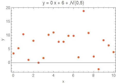
To explore this in a little more depth let's suppose that our data follows the equation $$y=\beta_1 x + \beta_0 + \mathcal{N}(0,\sigma)$$ where for concreteness $\beta_0=6$ and $\sigma=5$. Suppose also that we have a good scientific theoretical model that says $\beta_0 = 0$. Let's see what happens if we fit our data to 3 different models:

  1. An "overfitted" quadratic model: $y=\beta_2 x^2 + \beta_1 x + \beta_0 $
  2. The recommended "intercept" model: $y=\beta_1 x + \beta_0$
  3. The theoretical "no-intercept" model: $y=\beta_1 x$

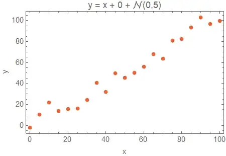
Let's sample 21 data points as follows:

Slope 1, intercept 6, data

Now, visually it seems that for $\beta_1=1$ and $\beta_0=6$ and $\sigma=5$ the small intercept is negligible, and the theoretical no-intercept model should be fine to use. The no-intercept model has an estimated $\beta_1 = 1.100 \ [1.044,1.157]$ which confidently excludes the true value of $1$. In contrast, the intercept model has an estimated $\beta_1 = 0.944 \ [0.874, 1.014]$ and the quadratic model has $\beta_1 = 1.091 \ [0.825, 1.358]$, both of which include the true value in the 95% confidence interval.

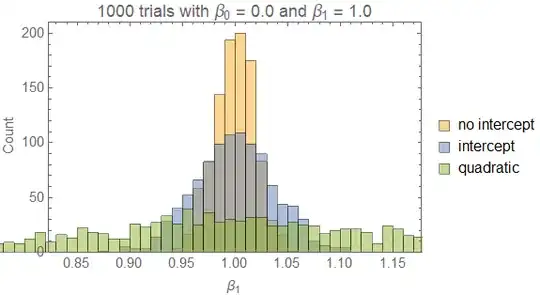
If we repeat this 1000 times we obtain the following histogram:

Slope 1, intercept 6, fit parameters

The intercept model is the best of these three, with the no-intercept model missing the true parameter in its confidence interval and the quadratic model having an overly broad confidence interval. This is confirmed by the Bayesian information criterion (BIC) which is lowest for the intercept model.

So one danger of the no-intercept model is the tendency to artificially introduce bias into the slope.


Another issue is the tendency to produce a statistically significant result even when there is no trend. To investigate this we will generate data with $\beta_1=0$ and $\beta_0=6$.

Slope 0, intercept 6, data

In this case the no-intercept model hallucinates a slope of $\beta_1=0.974 \ [0.521,1.428]$. Not only does this model invent a non-existent effect, it is quite confident, with a highly significant p-value of $p<0.001$, that the effect is non-zero. In contrast the intercept model obtains a non-significant ($p=0.792$) slope of $\beta_1 = 0.097 \ [-0.658,0.852]$, and the quadratic model obtains $\beta_1 = 1.892 \ [-0.951,4.735]$.

Again, repeating 1000 times we obtain

Slope 0, intercept 6, fit parameters

Again, the intercept model is the best of these three, with the no-intercept model missing the true parameter in its confidence interval and the quadratic model having an overly broad confidence interval. This is confirmed by the BIC which is again lowest for the intercept model.

So another danger of the no-intercept model is the tendency to artificially invent effects that do not exist, and to falsely produce such effects with a high degree of confidence.


Finally, let's examine the behavior of these models in the situation where the no-intercept model is actually appropriate. Here we will set $\beta_1=1$ and $\beta_0=0$ so the data actually matches the theoretical no-intercept model.

Slope 1, intercept 0, data

In this case all three models include the true slope of $1$ in the confidence interval. The no-intercept model estimates $\beta_1 = 1.021 \ [0.972,1.069]$ while the intercept model estimates $\beta_1 = 1.043 \ [0.947,1.139]$ and the quadratic model estimates $\beta_1 = 0.768 \ [0.415, 1.120]$.

Repeating this 1000 times we obtain the histogram:

Slope 1, intercept 0, fit parameters

This time, the no-intercept model is slightly better. All models provide an unbiased estimate of the $\beta_1$ parameter, but the no-intercept model has a slightly more narrow confidence interval. This is reflected in the fact that the no-intercept model has the lowest BIC of the three.

So, if a no-intercept model is desired, then an appropriate procedure would be to fit an intercept model, check the intercept, if it is not significant then fit the no-intercept model, and use some model-selection criterion to choose. But the first step will necessarily be to fit an intercept model. And often the extra steps are not worth the small improvement in precision gained with the no-intercept model.

Dale
  • 117,350
21

I cannot improve on Dale's answer, but speaking as an (ex) experimental scientist I strongly recommend you allow a non-zero intercept as it can be useful indication that you have systematic errors present.

We all learn how to estimate random errors, and in any case random errors are immediately apparent from the scatter in the points on the graph. However systemic errors can be a lot harder to spot, and getting an unexpectedly non-zero intercept is one indication they are present.

John Rennie
  • 367,598
5

My argument is that the model we have does not have a constant term and adding one would be overfitting so we should not fit to a=mz+b just like we shouldn't fit to a=mz2+bz+c. Another teacher argued that we should treat the data as the data and fit its true line of best fit, independent of what we think the model might be.

It depends on the hypothesis that you are testing and/or the kind of estimate you make. If, as you describe it, you have no reason to question the linear model, and the objective is estimating value of $g$, then there is no point of fitting $mz^2$ term - as you say, it would be overfitting.

This is largely true for the linear term, but linear term could be accounting for a systematic error, not captured by the model. On the other hand, if there is significant error in measurements, it would lead to significant overfitting, as in the figure below. Ultimately, this is a decision to make after the preliminary data examination.
enter image description here
(See When forcing intercept of 0 in linear regression is acceptable/advisable.)

With modern software, all three models could be easily tried and compared, and one could even use AIC or BIC criterion to test, which model overfits. There is a lot of statistics that one could learn from this simple experiment... but I suspect that this is not the objective of the physics class.

Remark
Answers by statisticians from the thread where I took the figure and the duplicate thread When is it ok to remove the intercept in a linear regression model? suggest that removing intercept in linear regression is rarely a good idea, although the reasons are somewhat more complex than overfitting/underfitting.

Note however, that from a statistician point of view, $a=mz^2+bz+c$ is still a linear model, but with an extra exploratory variable ($z^2$, it is linear in coefficients $m, b, c$, which can be easily found, e.g., using Ordinary least squares.) In this view adding an extra variable is not the same as adding an intercept.

Roger V.
  • 68,984
3

I write to add a central consideration that I do not see spelled out in the otherwise excellent answer by Dale. This is that one must be very cautious in using the standard statistical statements about goodness of fit and the likely range of fitted parameters. The statistical calculations that lead to things like a covariance matrix or a statement about the uncertainty of a gradient are based on the assumption that there is no systematic error at all. But this assumption is never fully correct and always dubious at best.

One way systematic error lurks is when the rule actually operating in the laboratory experiment is one formula (such as $y = a x + b$) but the rule you think is operating is another (such as $y = ax$). If you then fit your data using $y = ax$ then none of the standard statistical statements about how accurate your deduced gradient is can be trusted. The illustration treated by Dale gives a classic example of this: he invokes measures such as $p$ and reports confidence intervals based on using the $y = ax$ rule on data which was following another rule. But the value of $p$ and the confidence interval is then entirely misleading, because the assumptions underlying them in the statistical analysis do not hold.

The lesson I want to underline is that the case assumed in the standard statistical analysis is where the experimenter has the correct functional form for the dependence of some variable $y$ on some other variables $x_i$, and they are wishing to obtain good estimates of constant parameters in this function. But this situation is very rare in experimental science. Usually the laboratory equipment is doing one thing but you are guessing it is doing something else. That is, the experimenter guesses the data follows some law based on good physical reasoning, but the laboratory equipment is meanwhile responding to effects you never even thought of, including calibration and offset errors, aging or over-heating electronic circuitry, seismic noise, magnetic field noise, cosmic rays, non-linear response of materials, etc. etc.

If you want a good general-purpose way to find out how well your data is able to pin down a parameter in your model, look up the bootstrap method.

joseph h
  • 31,821
Andrew Steane
  • 65,285
2

A similar experiment with a spring and various weights would be modeled with Hooke's Law, which is $F=kx$. A plot of F vs. x yields a slope of $k$ and a y-intercept of 0. When actual data are taken and then plotted, it is often the case that a small amount of weight must be added to a real (aka non-ideal) spring before any spring extension is noted. This leads to a plot that has a positive y-intercept. Rather than forcing a y-intercept of 0, which would affect the slope of the plotted line and the calculated value of $k$, it is best to plot the data as measured and explain why the y-intercept is positive. In the case of a spring, particularly a new spring, there is some sort of "compression" created in the spring when it is manufactured, and that "compression" must be overcome before the spring shows any stretch. Thus, rather than forcing a y-intercept of 0, it is best to attempt an explanation of why the y-intercept is positive, and how real equipment differs from the assumptions made for ideal equipment. For the case of the Atwood's machine, there are undoubtedly friction, moments of inertia, etc., involved in the measurements that are not accounted for in the mathematical model being used.

David White
  • 12,602
1

Just as a practical matter, since all measuring instruments have both internal noise with some unknown bias, and moreover said bias can change unknowably with time, temperature, etc., one should always add the intercept in the model, if for no other reason then that it cannot hurt.

hyportnex
  • 21,193
0

I think it can be safely assumed that the experiment with $m_1=m_2$ was actually performed, and that the result $a=0$ was observed. Whether it actually was performed we don't know, but it is hard to conceive of an Attwood machine for which this would not have been true. Therefore the origin is a data point just as valid as any other. Fitting should allow for an offset, only in those cases where a plausible source of bias exists.