The CMB allows us to infer the value of $H_0$ because it provides us with a standard ruler, i.e. a feature which can be accurately measured and which has a physical size that can be computed from first principles. This is conceptual framework similar to the standard candle provided by the magnitude of type Ia supernovae.
The early universe was hot enough that the baryonic matter was fully ionized. The large density of free electrons meant that photons could readily Thomson scatter off of these electrons, and this interaction kept the radiation (photons) and matter tightly coupled in a primordial plasma. The matter distribution in the early universe was not entirely homogeneous due to fluctuations laid down during inflation. As such, there were gravitational potential wells and hills that this plasma could fall into. As the plasma fell in, it would compress and raise in temperature and pressure until the radiation pressure would be enough to cancel out the gravitational infall. In this way the plasma went through oscillations of compression and rarefaction known as acoustic oscillations.
As the universe expanded, it cooled down to the point that neutral hydrogen could begin to form, and relatively quickly the amount of free electrons in the universe dropped. Without a sufficient number of free electrons, photons no longer as readily interacted with the matter, and instead began to free stream without interactions. These free streaming photons from the primordial plasma are the CMB that we observe today.
The combination of the aforementioned oscillations and the decoupling of the photons from the plasma leads to a characteristic scale of spots that we see on the CMB. This is because a finite time elapsed between the big bang and decoupling. That is to say, there is a certain size such that photons that began gravitationally infalling at $t=0$ would have reached their maximum compression at the time of decoupling, and so we see these photons as a hot spot. The characteristic physical size of such a spot can be computed from first principles simply by considering the maximum distance that soundwave could travel in the plasma from $t=0$ to $t=t_d$, the time of decoupling. Mathematically, this is
$$
r_s = \int_0^t \frac{c_s(t)}{a(t)}dt = \int_{z_d}^\infty \frac{c_s(t)}{H(z)}dz
$$
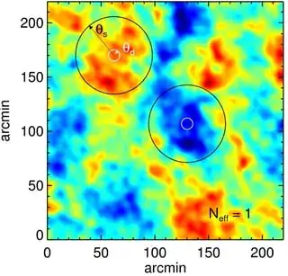
where $r_s$ is known as the comoving sound horizon. This is the physical size of a "typical spot" on the CMB, as demonstrated in this figure from [1]
When we observe the CMB, we can very accurately measure the angular scale of these spots, and on theoretical grounds we can calculate what their physical size must be. The relationship between angular size and physical size is familiar from standard trigonometry, $r_s = \theta_s D_A$, where $D_A$ is a quantity known as the angular diameter distance and can be thought of as a measure of distance between us and the surface of last scattering, i.e. the distance between us and where the CMB photons we are observing had their last interaction. This distance is related to the expansion history of the universe between now and last scattering: a quicker expansion means that this surface of last scattering is closer. This is because quicker expansion means that it has not taken the universe as long to reach its current size, and so the CMB photons have had less time to travel and as such must have originated closer. Mathematically this relationship is:
$$
D_A = \int_0^{z_d} \frac{dz}{H(z)}
$$
Since we know $r_s$ and can measure $\theta_s$, then we know what the left hand side of the above expression is, and as such can find the right hand side, i.e. we can determine $H(z)$ for all $z$ including $z=0$, which would be $H_0$. This inference is model dependent - it depends on how $H(z)$ is related to the ingredients of the universe, i.e. it depends on the functional form of the integrand above. So if we assume a model like $\Lambda$CDM, we can make an inference as to the expansion rate today. But changing that assumption may change the inference. This is why the discrepancy between CMB and local universe measurements is exciting to many cosmologists. If it is a real discrepancy, it suggests that we may need to change that assumption so that the inference from CMB data is consistent with local universe measurements.
I have left out many, many details in the above. For further reading I recommend section II of the Hubble Hunter's Guide, Knox and Millea
EDIT:
There have been some questions as to why the dependence on $H_0$ does not simply cancel in the expression for the angular size of the sound horizon. I gave a brief, perhaps too brief, reply in the comments which I am expanding on here.
The first thing I will say is that the acoustic scale indeed does not depend on $H_0$, so in that sense it does cancel. We cannot learn about $H_0$ only from $\theta_{\star}$ unless, and this is crucial, we have some information about either $r_s$ or $D_A$. From our understanding of the relatively simply physics of acoustic oscillations in the primordial plasma, we know theoretically what $r_s$ must be, and therefore we can learn something about $H_0$. To see this more explicitly, consider that:
$$
H^2(z) = \frac{8 \pi G}{3} \left(\rho_m(z) + \rho_r(z) + \rho_{\Lambda}(z) \right)
$$
A common way to express the densities on the right hand side is in units of "the critical density of a $H_0 = 100 \text{ km/s/Mpc}$ universe", that is in units of $\rho_{\rm c,100} \equiv \frac{3 \left( 100 \text{ km/s/Mpc}\right)^2}{8 \pi G}$. We denote $\rho_i / \rho_{\rm c,100} = \omega_i$ and call it the physical density of component $i$, since that's what it is, just expressed in weird units.
Now, we define $H(z)/\left(100 \text{ km/s/Mpc} \right) \equiv h(z)$ and we can write the above expression as
$$
h(z) = 2998 \text{ Mpc} \sqrt{\omega_m(z) + \omega_r(z) + \omega_\Lambda}
$$
The dependence on $H_0$ has been hidden in the left hand side, but I feel this makes what happens a bit more clear. The entire above discussion and be rephrased and summarized as:
- At early times, $\omega_{\Lambda}$ is negligible so $h(z)$ only depends on $\omega_m = \omega_c + \omega_b$ and $\omega_r$ at early times. The CMB temperature tells us $\omega_r$, and we can infer $\omega_c$ and $\omega_b$ from the CMB power spectrum alone, or in combination with BBN data. These observations directly tell us about the expansion rate at early times, and allow us to compute $r_s$.
- We measure $\theta_s$, which is independent of $H_0$ because the dependence there cancels out as noted in the comments.
- At late times, $h(z)$ now depends on $\omega_\Lambda$ as dark energy has become dominant. It is the only remaining thing that we can adjust, so we adjust it so that we get the observed $\theta_s$ given the theoretically calculated $r_s$. If you'd like, the observed $\theta_s$ in a sense tells us the conversion factor from early time $H(z)$ to $H(z)$ today.
With $\omega_m$, $\omega_r$ and $\omega_\Lambda$ determined, we have determined $h(z)$ at all redshifts including at $z=0$, and hence $H_0$. A final summary: $r_s$ only depends on the early time expansion history, which is basically independent of $\rho_\Lambda$. For a fixed early expansion history, we could have many different expansion rates today depending on what the value of $\rho_\Lambda$ is. We can fix the early expansion history by learning $\rho_m$ from the CMB power spectrum and $\rho_r$ from the CMB temperature. It is these measurements which give us knowledge of the expansion rate. We translate those into a constraint on the expansion rate today using an observation of $\theta_s$. Given a fixed early expansion rate history, there is only one value of $\rho_\Lambda$ which gives us the observed $\theta_s$, and hence the rate today. I hope this helps.
