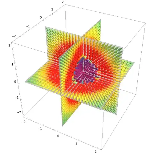
By using inverse square with 3D as suggested, we get the following:
$$\sum_{p\in P} \left<\frac{x-p_x} {\sqrt{(x-p_x)^2 + (y-p_y)^2 + (z-p_z)^2} ^3} , \frac{y-p_y} {\sqrt{(x-p_x)^2 + (y-p_y)^2 + (z-p_z)^2} ^3}, \frac{z-p_z} {\sqrt{(x-p_x)^2 + (y-p_y)^2 + (z-p_z)^2}^3}\right>$$
m = SpherePoints[250];
f[p_] := 0.01*((x-p[[1]])/(((x-p[[1]])^2+(y-p[[2]])^2 + (z-p[[3]])^2)^(3/2)));
g[p_] := 0.01*((y-p[[2]])/(((x-p[[1]])^2+(y-p[[2]])^2 + (z-p[[3]])^2)^(3/2)));
h[p_] := 0.01*((z-p[[3]])/(((x-p[[1]])^2+(y-p[[2]])^2 + (z-p[[3]])^2)^(3/2)));
SliceVectorPlot3D[{Total[Map[f, m]], Total[Map[g, m]], Total[Map[h, m]]}, "CenterPlanes", {x, -2, 2}, {y, -2,2}, {z, - 2,2}, VectorColorFunction -> (ColorData["Rainbow"][#7]&) , PlotLegends -> BarLegend["Rainbow"], VectorColorFunctionScaling -> False, VectorRange -> All, VectorPoints -> 25, ImageSize -> {500,500}]
With 2D it requires reverse linear to get the expected result of no field inside the circle:
$$\sum_{p\in P} \left<\frac{x-p_x} {(x-p_x)^2 + (y-p_y)^2} , \frac{y-p_y} {(x-p_x)^2 + (y-p_y)^2}\right>$$
m = CirclePoints [125];
f[p_] := 0.01*((x-p[[1]])/(((x-p[[1]])^2+(y-p[[2]])^2)^(2/2)));
g[p_] := 0.01*((y-p[[2]])/(((x-p[[1]])^2+(y-p[[2]])^2)^(2/2)));
VectorPlot[{Total[Map[f, m]], Total[Map[g, m]]} , {x, -2, 2}, {y, -2,2}, VectorColorFunction -> (ColorData["Rainbow"][#5]&) , PlotLegends -> BarLegend["Rainbow"], VectorColorFunctionScaling -> False, VectorRange -> All, VectorPoints -> 50, ImageSize -> {500,500}]
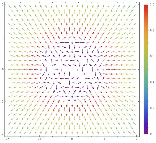
Red in these plots means anything over 1. The first equation looks like inverse cube but it's actually inverse square because you need to normalise the vector first, which involves another division by r.


