Firstly, in your code you are confusing wavelength with frequency. You defined $\omega_0$ as 1µm. That is a typical wavelength ($\lambda$).
$\omega=\frac{2\pi c}{\lambda}$
For 1µm wavelengths you need your time axis to be in the femtoseconds to be able to see the electric field. I see now another point of confusion. You are defining things in the spatial domain with nanometer precision instead of doing it in the time domain: chirp is typically defined in time, not in space (of course that for a fixed time, in space you would also see a "chirp", but of wavelength, however chirp comes from a time-varying instantaneous frequency.)
Secondly, it appears to me that your chirp is ill defined, in the sense that you are adding frequencies that are beating under your envelope. But that is just from taking a quick look at the image.
However, instead of doing it in the time domain, do it instead in the frequency domain:
Define $A(\omega)$ as the amplitude envelope. For example a Gaussian centered at your frequency of interest. Define $\omega_0$ correctly.
Then just multiply by a phase term: $e^{i\phi(\omega)}$
Where you define $\phi(\omega)$ from the taylor expansion of the phase.
For a simple chirp:
$\phi(\omega)=\frac{1}{2}GDD(\omega-\omega_0)^2$
Where GDD is the group delay dispersion.
Then just do the inverse Fourier transform of the spectral definition of your pulse.
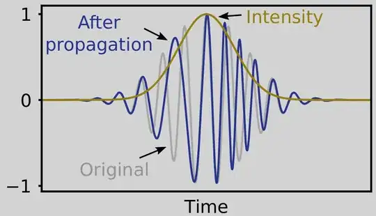
Plotting the real part will give you the E-field oscillations and plotting the absolute square will give you the power envelope.
You will get then the same image as the one from RP photonics (if you plot the square root of the absolute square, to represent the envelope of the E-field and not of the power).
The image below was obtained like that.
(To be honest, the image is SPM not just chirp, but the concept is the same, I'm too tired to make an illustrative image with just chirp.)