When you apply Huygen's principle you also have to think about all the different phases that might constructively or destructively interfere. An infinite plane wave is one example where the region of constructive interference is easy to think about but generally it will be much harder. That being said, plane waves that are not infinitely long do spread out a little. How much depends on the wavelength and extent of the wave. If the wavelength is small compared to the extent (i.e. it is generated by a large slit) the wave will move relatively straight. In the opposite limit if the slit is very small the wave will spread out like a point source. Using Mathematica I was able to make the following animation:
The final frame looks like this top down:
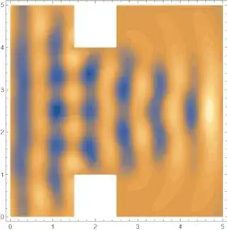
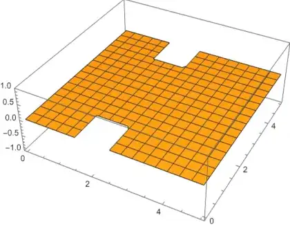
The left boundary generates sine waves, all the other boundaries are absorbing except for the two linepieces on the inside of the gap which are hard boundaries.
I used the following code to generate the animation
H = 5;
L = 5;
T = 5;
\[Delta] = .5;
a = H*.3;
box = Region[Rectangle[ {0, 0}, {L, H}]];
wall1 = Region[Rectangle[ {2 - \[Delta], 0}, {2 + \[Delta], H/2 - a}]];
wall2 = Region[Rectangle[ {2 - \[Delta], H/2 + a}, {2 + \[Delta], H}]];
region = RegionDifference[box, wall1];
region = RegionDifference[region, wall2];
\[Sigma] = .2;
wave2D = NDSolveValue[{D[u[t, x, y], {t, 2}] -
      Laplacian[u[t, x, y], {x, y}] ==
     NeumannValue[-Derivative[1, 0, 0][u][t, x, y], x != 0] +
      NeumannValue[1.5 Sin[8 t], x == 0],
    u[0, x, y] == 0,
    DirichletCondition[u[t, x, y] == 0,
     x > 0 && x < L && y >= H/2 - a - .01 && y <= H/2 + a + .01],
    Derivative[1, 0, 0][u][0, x, y] == 0
    }, u, {t, 0, T}, {x, y} \[Element] region];
plot = Table[
   Plot3D[wave2D[t, x, y], {x, 0, L}, {y, 0, H}, PlotRange -> {-1, 1},
     BoxRatios -> Automatic], {t, 0, T, .1}];
ListAnimate[plot]


