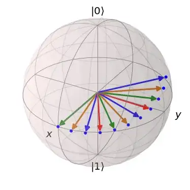
How do I visualize a stepwise rotation on the Bloch Sphere using $SO(3)$ and $SU(2)$?

Question

Searching for an implementation (that helps me to understand how $SO(3)$ and $SU(2)$ relate to each other) I came across this interesting question Visual interpretation, on the Bloch sphere, when Hadamard gate is applied twice where qutip is utilized. However my question is more fundamental.

Using qutip too, I implemented a rotation of a Qubit on a Bloch Sphere using $SO(3)$ as follows:

import qutip as qt
from qutip.qip.operations import rx
import numpy as np
def to_spherical(state):
    r0 = np.abs(state[0])
    ϕ0 = np.angle(state[0])
    r1 = np.abs(state[1])
    ϕ1 = np.angle(state[1])
    r = np.sqrt(r0 ** 2 + r1 ** 2)
    θ = 2 * np.arccos(r0 / r)
    ϕ = ϕ1 - ϕ0
    return [r, θ, ϕ]
def to_cartesian(polar):
    r = polar[0]
    θ = polar[1]
    ϕ = polar[2]
    x = r * np.sin(θ) * np.cos(ϕ)
    y = r * np.sin(θ) * np.sin(ϕ)
    z = r * np.cos(θ)
    return [x, y, z]
def rn_so3(state, theta, phi, delta):
    rn_mat = qt.Qobj(
        [[np.cos(delta/2) - (0+1j)np.cos(theta)np.sin(delta/2),
          -(0+1j)np.exp(-(0+1j)phi)np.sin(delta/2)np.sin(theta)],
         [-(0+1j)np.exp((0+1j)phi)np.sin(delta/2)np.sin(theta),
          np.cos(delta/2) + (0+1j)np.cos(theta)np.sin(delta/2)]]
        )
    r_state = (rn_matstate)(rn_mat*state).dag()
    return(r_state)
b = qt.Bloch()
b.clear()
b.make_sphere()
states = []
points = []
alpha = 1/np.sqrt(2)
beta = 1/np.sqrt(2)
s = np.array([alpha,beta])
state = qt.Qobj(s)
states.append(state)
Ψ = [complex(alpha, 0), complex(beta, 0)]
polar = to_spherical(Ψ)
pnt = to_cartesian(polar)
points.append(pnt)
rotated = state
for i in range(0,10):
    rotated = rn_so3(rotated, 0.4, 0.3, 0.2)
    pnt = [(qt.sigmax()rotated).tr(), (qt.sigmay()rotated).tr(), (qt.sigmaz()*rotated).tr()]
    states.append(rotated)
    points.append(pnt)
b.add_states(states)
np_points = np.array(points)
b.add_points([np_points[:,0], np_points[:,1], np_points[:,2]])
b.show()

The corresponding output looks as follows:

My question: Can I achieve the same output using the $SU(2)$ group and coordinate transformations?

I found also the formula for the rotation around an axis on the Bloch Sphere with an angle $\theta$ that looks as follows:

$$R_A(\theta)=\cos\frac{\theta}{2}\sigma_I-i\cdot\sin\frac{\theta}{2}(x_A\sigma_x+y_A\sigma_y+z_A\sigma_z)$$ which I tried to implement too but didn't output the desired rotation.

My trial looks as follows and I am trying to refer to this document "Lecture notes: Qubit representations and rotations":

def rn_su2(θ, ϕ):
    return (np.sin(θ)*np.cos(ϕ)*qt.sigmax() + np.sin(θ)*np.sin(ϕ)*qt.sigmay() + np.cos(θ)*qt.sigmaz())
b = qt.Bloch()
b.clear()
b.make_sphere()
states = []
points = []
alpha = 1/np.sqrt(2)
beta = 1/np.sqrt(2)
s = np.array([alpha,beta])
state = qt.Qobj(s)
states.append(state)
Ψ = [complex(alpha, 0), complex(beta, 0)]
polar = to_spherical(Ψ)
pnt = to_cartesian(polar)
points.append(pnt)
rotated = state
for i in range(0,10):
    #
    # Here seems to go something wrong
    #
    rotated = rn_su2(0.2i, 0.3i)
    states.append(rotated)
#polar = to_spherical(rotated)
#pnt = to_cartesian(polar)    
points.append(pnt)


b.add_states(states)
np_points = np.array(points)
b.add_points([np_points[:,0], np_points[:,1], np_points[:,2]])
b.show()

Here I have some fundamental error and would appreciate any help or hint.

Update 2022-03-19: I implemented the $SU(2)$ rotation according the useful hint in the comment. It looks better, but unfortunatelly the state lies not on the Bloch Sphere anymore:

def rn_su2(θ, state, nx, ny, nz):
    Ψ = [state.data[0,0], state.data[1,0]]
    arr = to_spherical(Ψ)
    s_θ = arr[1]
    s_ϕ = arr[2]
    M_q = np.sin(s_θ)*np.cos(s_ϕ)*qt.sigmax() + np.sin(s_θ)*np.sin(s_ϕ)*qt.sigmay() + np.cos(s_θ)*qt.sigmaz()
    U_n = qt.qeye(2)*np.cos(θ/2) -1j*(nx*qt.sigmax()+ny*qt.sigmay()+nz*qt.sigmaz())*np.sin(θ/2)
    r_state = U_n*M_q*U_n.dag()
    return r_state

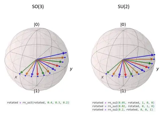
Update 2022-03-20: After fixing the $SU(2)$ rotations code it looks good and correct. Now I'm just struggling with the actual question: what angles do I need to use so that both plots (vertex sequences) look the same? In the $SO(3)$ implementation case I used rotated = rn_so3(rotated, 0.4, 0.3, 0.2) and to get an almost same looking picture, by trial and error, I obtained for the $SU(2)$ implementation:

rotated = rn_su2(0.05, rotated, 1, 0, 0)
rotated = rn_su2(0.02, rotated, 0, 1, 0)
rotated = rn_su2(0.2, rotated, 0, 0, 1)

The comparative figures are as follows:

How do I visualize a stepwise rotation on the Bloch Sphere using $SO(3)$ and $SU(2)$?

0 Answers0