Poisson-Nearst-Planck equations with normal distribution as initial condition

Question

I am having a hard time trying to think of this model:

Imagine you have a normal distribution of +q charges in 2D

$$\rho(r,t=0)=\rho_0 e^{-\frac{r^2}{\sigma_0^2}} $$

where $\sigma_0$ is the width of the distribution. How does the distribution change over time?

To model this, Nearst-Planck equation can be written as

$$\frac{\partial }{\partial t}\rho(t,r)=D[\nabla^2\rho(r,t)-\beta \nabla\cdot(\textbf{E}(r,t)\rho(r,t))]$$ with D as the diffusion coefficient and $\beta=(kT)^{-1}$ as the reciprocal of the thermodynamic temperature. The $\textbf{E}$ field is due to the charge distribution itself. But

$$\textbf{E}(r,t)=-\nabla \phi(r,t) $$

so the equation is rewritten as

$$\frac{\partial }{\partial t}\rho(t,r)=D[\nabla^2\rho(r,t)+\beta \nabla\cdot(\nabla \phi(r,t)\rho(r,t))]$$

Additionally, due to Poisson's equation

$$\nabla^2\phi=-\frac{\rho(r,t)}{\epsilon}$$

It is known that for non-charged-particles ($\phi=0$), the solution for the same initial condition (normal distribution) is:

$$ \rho(r,t)=\frac{\rho_0 \sigma_0^2}{\sigma_0^2+4Dt}e^{-\frac{r^2}{\sigma_0^2+4Dt}}$$ which is just a Gaussian with a width $(\sigma_0^2+4Dt)^{\frac{1}{2}}$.

Is it possible to try to approximate the solution or simulate numerically the distribution over time for charged particles?

Thanks for all the insights!

Answer 1

It seems to me that the problem you will run into is not that you have a $\rho^2$ term (easily addressed since $\rho(x_i)\to\rho_i\implies\rho(x_i)^2=\rho_i^2$; consider, for instance, the Burgers' equation), but that you will end up with a term like $\nabla\phi\cdot\nabla\rho$, so the potential will need to be tracked and evolved, which means you have a pair of diffusion problems to solve at each step, which is time-consuming computationally--though this means it should be solvable numerically.

Essentially, your simulation would be something like,

1. Initialize $\rho(r,\,0)$
2. Compute $\phi(r,\,0)$ using the Poisson equation
3. Evolve $\rho(r,\,\mathrm{d}t)$ using the Nearst-Planck equation
4. Continue from #2 until required $t$ is satisfied.

Presumably you would use escaping boundaries, but whatever boundaries you choose would be applied with each step.

In Cartesian coordinates, the discretization scheme should be pretty straight-forward, e.g., for 1D you'd have, $$ \frac{\rho_{i}^{n+1}-\rho_{i}^n}{\mathrm{d}t}=D\left[\frac{\rho_{i+1}^n+\rho_{i-1}^n-2\rho_i^n}{\mathrm{d}x^2}-\frac{\beta}{\varepsilon}\left(\rho_i^n\right)^2+\frac{\beta}{4}\frac{\phi_{i+1}-\phi_{i-1}}{\mathrm{d}x}\cdot\frac{\rho_{i+1}^n-\rho_{i-1}^n}{\mathrm{d}x}\right].\tag{1} $$ Though, if you intend on using the radial form, you may run into the issue of dividing by zero with the diffusion term. This can be mitigated by other means, as I discuss in this post of mine. But I otherwise don't see any issues that could arise in solving the system.

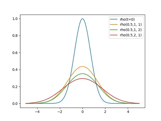
I used Eq (1) with a couple different parameters of $\rho\left(t,\,D,\,\beta\right)$ (though with $\sigma_0=\varepsilon=1$) for $x\in[-5,\,5]$ and ran it from $t=0$ until $t=0.5$ and found the following,
which looks still reasonably Gaussian for the different parameter pairs. It appears that $\beta$ is controls the height of the central peak while $D$ controls the width and heights.

^{The Python code I used to produce the above can be found in my github page.}